![]()
![]() "
]
},
{
"cell_type": "markdown",
"metadata": {
"nbpages": {
"level": 1,
"link": "[3.3 Linear Approximation of a Multivariable Model](https://jckantor.github.io/CBE30338/03.03-Linear-Approximation-of-a-Multivariable-Model.html#3.3-Linear-Approximation-of-a-Multivariable-Model)",
"section": "3.3 Linear Approximation of a Multivariable Model"
}
},
"source": [
"# 3.3 Linear Approximation of a Multivariable Model"
]
},
{
"cell_type": "markdown",
"metadata": {
"nbpages": {
"level": 2,
"link": "[3.3.1 Multivariable Systems](https://jckantor.github.io/CBE30338/03.03-Linear-Approximation-of-a-Multivariable-Model.html#3.3.1-Multivariable-Systems)",
"section": "3.3.1 Multivariable Systems"
}
},
"source": [
"## 3.3.1 Multivariable Systems"
]
},
{
"cell_type": "markdown",
"metadata": {
"nbpages": {
"level": 2,
"link": "[3.3.1 Multivariable Systems](https://jckantor.github.io/CBE30338/03.03-Linear-Approximation-of-a-Multivariable-Model.html#3.3.1-Multivariable-Systems)",
"section": "3.3.1 Multivariable Systems"
}
},
"source": [
"Most process models consist of more than a single state and a single input. Techniques for linearization extend naturally to multivariable systems. The most convenient mathematical tools involve some linear algebra."
]
},
{
"cell_type": "markdown",
"metadata": {
"nbpages": {
"level": 3,
"link": "[3.3.1.1 Example: Gravity Drained Tanks](https://jckantor.github.io/CBE30338/03.03-Linear-Approximation-of-a-Multivariable-Model.html#3.3.1.1-Example:-Gravity-Drained-Tanks)",
"section": "3.3.1.1 Example: Gravity Drained Tanks"
}
},
"source": [
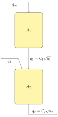
"### 3.3.1.1 Example: Gravity Drained Tanks\n",
"\n",
"Here we develop a linear approximation to a process model for a system consisting of coupled gravity-drained tanks. \n",
"\n",
""
]
},
{
"cell_type": "markdown",
"metadata": {
"nbpages": {
"level": 4,
"link": "[3.3.1.1.1 Model](https://jckantor.github.io/CBE30338/03.03-Linear-Approximation-of-a-Multivariable-Model.html#3.3.1.1.1-Model)",
"section": "3.3.1.1.1 Model"
}
},
"source": [
"#### 3.3.1.1.1 Model\n",
"\n",
"\\begin{eqnarray*}\n",
"A_{1}\\frac{dh_{1}}{dt} & = & q_{in}-C_{1}\\sqrt{h_{1}}\\\\\n",
"A_{2}\\frac{dh_{2}}{dt} & = & q_{d}+C_{1}\\sqrt{h_{1}}-C_{2}\\sqrt{h_{2}}\n",
"\\end{eqnarray*}"
]
},
{
"cell_type": "markdown",
"metadata": {
"nbpages": {
"level": 4,
"link": "[3.3.1.1.2 Nominal Inputs](https://jckantor.github.io/CBE30338/03.03-Linear-Approximation-of-a-Multivariable-Model.html#3.3.1.1.2-Nominal-Inputs)",
"section": "3.3.1.1.2 Nominal Inputs"
}
},
"source": [
"#### 3.3.1.1.2 Nominal Inputs\n",
"\n",
"\\begin{eqnarray*}\n",
"\\bar{q}_{in} & = & \\bar{q}_{in}\\\\\n",
"\\bar{q}_{d} & = & 0\n",
"\\end{eqnarray*}"
]
},
{
"cell_type": "markdown",
"metadata": {
"nbpages": {
"level": 4,
"link": "[3.3.1.1.3 Steady State for nominal input](https://jckantor.github.io/CBE30338/03.03-Linear-Approximation-of-a-Multivariable-Model.html#3.3.1.1.3-Steady-State-for-nominal-input)",
"section": "3.3.1.1.3 Steady State for nominal input"
}
},
"source": [
"#### 3.3.1.1.3 Steady State for nominal input\n",
"\n",
"\\begin{eqnarray*}\n",
"\\bar{h}_{1} & = & \\frac{\\bar{q}_{in}^{2}}{C_{1}^{2}}\\\\\n",
"\\bar{h}_{2} & = & \\frac{\\bar{q}_{in}^{2}}{C_{2}^{2}}\n",
"\\end{eqnarray*}"
]
},
{
"cell_type": "markdown",
"metadata": {
"nbpages": {
"level": 4,
"link": "[3.3.1.1.4 Deviation Variables](https://jckantor.github.io/CBE30338/03.03-Linear-Approximation-of-a-Multivariable-Model.html#3.3.1.1.4-Deviation-Variables)",
"section": "3.3.1.1.4 Deviation Variables"
}
},
"source": [
"#### 3.3.1.1.4 Deviation Variables\n",
"\n",
"States\n",
"\n",
"\\begin{eqnarray*}\n",
"x_{1} & = & h_{1}-\\bar{h}_{1}\\\\\n",
"x_{2} & = & h_{2}-\\bar{h}_{2}\n",
"\\end{eqnarray*}\n",
"\n",
"Control input\n",
"$$u=q_{in}-\\bar{q}_{in}$$\n",
"\n",
"Disturbance input\n",
"$$d=q_{d}-\\bar{q}_{d}$$\n",
"\n",
"Measured output\n",
"$$y=h_{2}-\\bar{h}_{2}$$"
]
},
{
"cell_type": "markdown",
"metadata": {
"nbpages": {
"level": 4,
"link": "[3.3.1.1.5 Linearization ](https://jckantor.github.io/CBE30338/03.03-Linear-Approximation-of-a-Multivariable-Model.html#3.3.1.1.5-Linearization)",
"section": "3.3.1.1.5 Linearization "
}
},
"source": [
"#### 3.3.1.1.5 Linearization \n",
"\n",
"\\begin{eqnarray*}\n",
"\\frac{dh_{1}}{dt} & = & \\frac{1}{A_{1}}\\left(q_{in}-C_{1}\\sqrt{h_{1}}\\right)=f_{1}(h_{1},h_{2},q_{in},q_{d})\\\\\n",
"\\frac{dh_{2}}{dt} & = & \\frac{1}{A_{2}}\\left(q_{d}+C_{1}\\sqrt{h_{1}}-C_{2}\\sqrt{h_{2}}\\right)=f_{2}(h_{1},h_{2},q_{in},q_{d})\n",
"\\end{eqnarray*}\n",
"\n",
"Taylor series expansion for the first tank\n",
"\n",
"\\begin{eqnarray*}\n",
"\\frac{dx_{1}}{dt} & = & f_{1}(\\bar{h}_{1}+x_{1},\\bar{h}_{2}+x_{2},\\bar{q}_{in}+u,\\bar{q}_{d}+d)\\\\\n",
" & \\approx & \\underbrace{f_{1}(\\bar{h}_{1},\\bar{h}_{2},\\bar{q}_{in})}_{0}+\\left.\\frac{\\partial f_{1}}{\\partial h_{1}}\\right|_{SS}x_{1}+\\left.\\frac{\\partial f_{1}}{\\partial h_{2}}\\right|_{SS}x_{2}+\\left.\\frac{\\partial f_{1}}{\\partial q_{in}}\\right|_{SS}u+\\left.\\frac{\\partial f_{1}}{\\partial q_{d}}\\right|_{SS}d\\\\\n",
" & \\approx & \\left(-\\frac{C_{1}}{2A_{1}\\sqrt{\\bar{h}_{1}}}\\right)x_{1}+\\left(0\\right)x_{2}+\\left(\\frac{1}{A_{1}}\\right)u+\\left(0\\right)d\\\\\n",
" & \\approx & \\left(-\\frac{C_{1}^{2}}{2A_{1}\\bar{q}_{in}}\\right)x_{1}+\\left(\\frac{1}{A_{1}}\\right)u\n",
"\\end{eqnarray*}\n",
"\n",
"Taylor series expansion for the second tank\n",
"\n",
"\\begin{eqnarray*}\n",
"\\frac{dx_{2}}{dt} & = & f_{2}(\\bar{h}_{1}+x_{1},\\bar{h}_{2}+x_{2},\\bar{q}_{in}+u,\\bar{q}_{d}+d)\\\\\n",
" & \\approx & \\underbrace{f_{2}(\\bar{h}_{1},\\bar{h}_{2},\\bar{q}_{in})}_{0}+\\left.\\frac{\\partial f_{2}}{\\partial h_{1}}\\right|_{SS}x_{1}+\\left.\\frac{\\partial f_{2}}{\\partial h_{2}}\\right|_{SS}x_{2}+\\left.\\frac{\\partial f_{2}}{\\partial q_{in}}\\right|_{SS}u+\\left.\\frac{\\partial f_{2}}{\\partial q_{d}}\\right|_{SS}d\\\\\n",
" & \\approx & \\left(\\frac{C_{1}}{2A_{2}\\sqrt{\\bar{h}_{1}}}\\right)x_{1}+\\left(-\\frac{C_{2}}{2A_{2}\\sqrt{\\bar{h}_{2}}}\\right)x_{2}+\\left(0\\right)u+\\left(\\frac{1}{A_{2}}\\right)d\\\\\n",
" & \\approx & \\left(\\frac{C_{1}^{2}}{2A_{2}\\bar{q}_{in}}\\right)x_{1}+\\left(-\\frac{C_{2}^{2}}{2A_{2}\\bar{q}_{in}}\\right)x_{2}+\\left(\\frac{1}{A_{2}}\\right)d\n",
"\\end{eqnarray*}\n",
"\n",
"Measured outputs\n",
"\n",
"\\begin{eqnarray*}\n",
"y & = & h_{2}-\\bar{h}_{2}\\\\\n",
" & = & x_{2}\n",
"\\end{eqnarray*}"
]
},
{
"cell_type": "markdown",
"metadata": {
"nbpages": {
"level": 4,
"link": "[3.3.1.1.6 Summary of the linear model using matrix/vector notation](https://jckantor.github.io/CBE30338/03.03-Linear-Approximation-of-a-Multivariable-Model.html#3.3.1.1.6-Summary-of-the-linear-model-using-matrix/vector-notation)",
"section": "3.3.1.1.6 Summary of the linear model using matrix/vector notation"
}
},
"source": [
"#### 3.3.1.1.6 Summary of the linear model using matrix/vector notation\n",
"\n",
"\\begin{eqnarray*}\n",
"\\frac{d}{dt}\\left[\\begin{array}{c}\n",
"x_{1}\\\\\n",
"x_{2}\n",
"\\end{array}\\right] & = & \\left[\\begin{array}{cc}\n",
"-\\frac{C_{1}^{2}}{2A_{1}\\bar{q}_{in}} & 0\\\\\n",
"\\frac{C_{1}^{2}}{2A_{2}\\bar{q}_{in}} & -\\frac{C_{2}^{2}}{2A_{2}\\bar{q}_{in}}\n",
"\\end{array}\\right]\\left[\\begin{array}{c}\n",
"x_{1}\\\\\n",
"x_{2}\n",
"\\end{array}\\right]+\\left[\\begin{array}{c}\n",
"\\frac{1}{A_{1}}\\\\\n",
"0\n",
"\\end{array}\\right]u+\\left[\\begin{array}{c}\n",
"0\\\\\n",
"\\frac{1}{A_{2}}\n",
"\\end{array}\\right]d\\\\\n",
"y & = & \\left[\\begin{array}{cc}\n",
"0 & 1\\end{array}\\right]\\left[\\begin{array}{c}\n",
"x_{1}\\\\\n",
"x_{2}\n",
"\\end{array}\\right]+\\left[\\begin{array}{c}\n",
"0\\end{array}\\right]u+\\left[\\begin{array}{c}\n",
"0\\end{array}\\right]d\n",
"\\end{eqnarray*}"
]
},
{
"cell_type": "markdown",
"metadata": {
"nbpages": {
"level": 2,
"link": "[3.3.2 Exercises](https://jckantor.github.io/CBE30338/03.03-Linear-Approximation-of-a-Multivariable-Model.html#3.3.2-Exercises)",
"section": "3.3.2 Exercises"
}
},
"source": [
"## 3.3.2 Exercises"
]
},
{
"cell_type": "markdown",
"metadata": {
"nbpages": {
"level": 3,
"link": "[3.3.2.1 First Order Reaction in a CSTR](https://jckantor.github.io/CBE30338/03.03-Linear-Approximation-of-a-Multivariable-Model.html#3.3.2.1-First-Order-Reaction-in-a-CSTR)",
"section": "3.3.2.1 First Order Reaction in a CSTR"
}
},
"source": [
"### 3.3.2.1 First Order Reaction in a CSTR\n",
"A first-order reaction\n",
"\n",
"$$A\\longrightarrow\\mbox{Products}$$\n",
"takes place in an isothermal CSTR with constant volume $V$, volumetric\n",
"flowrate in and out the same value $q$, reaction rate constant $k$,\n",
"and feed concentration $c_{AF}$.\n",
"\n",
"* Write the material balance equation for this system as a first-order ordinary differential equation. \n",
"* Algebraically determine the steady-state solution to this equation. \n",
"* For what values of $q$, $k$, $V$, and $c_{AF}$ is this stable?\n",
"* For a particular reaction $k$ = 2 1/min. We run this reaction in a vessel of volume $V$ =10 liters, volumetric flowrate $q$ = 50 liters/min. The desired exit concentrationof $A$ is $0.1$ gmol/liter. Assume that we can manipulate $c_{AF}$, the concentration of $A$ entering the CSTR, with proportional control, in order to control the concentration of $A$ exiting the reactor. Substitute the appropriate control law into the mathematical model and rearrange it to get a model of the same form as part (a).\n",
"* Determine the steady-state solution to this equation. If we set $K_{c}=100$, what is the absolute value of the offset between the exit concentration of $A$ and the desired exit concentration of $A$? "
]
},
{
"cell_type": "markdown",
"metadata": {
"nbpages": {
"level": 3,
"link": "[3.3.2.2 Two Gravity Drained Tanks in Series](https://jckantor.github.io/CBE30338/03.03-Linear-Approximation-of-a-Multivariable-Model.html#3.3.2.2-Two-Gravity-Drained-Tanks-in-Series)",
"section": "3.3.2.2 Two Gravity Drained Tanks in Series"
}
},
"source": [
"### 3.3.2.2 Two Gravity Drained Tanks in Series\n",
"Consider the two-tank model. Assuming the tanks are identical, and\n",
"using the same parameter values as used for the single gravity-drained\n",
"tank, compute values for all coefficients appearing in the multivariable\n",
"linear model. Is the system stable? What makes you think so? "
]
},
{
"cell_type": "markdown",
"metadata": {
"nbpages": {
"level": 3,
"link": "[3.3.2.3 Isothermal CSTR with second-order reaction](https://jckantor.github.io/CBE30338/03.03-Linear-Approximation-of-a-Multivariable-Model.html#3.3.2.3-Isothermal-CSTR-with-second-order-reaction)",
"section": "3.3.2.3 Isothermal CSTR with second-order reaction"
}
},
"source": [
"### 3.3.2.3 Isothermal CSTR with second-order reaction\n",
"Consider an isothermal CSTR with a single reaction \n",
"$$A\\longrightarrow\\mbox{Products}$$\n",
"whose reaction rate is second-order. Assume constant volume, $V$,\n",
"and density, $\\rho$, and a time-dependent volumetric flow rate $q(t)$.\n",
"The input to the reactor has concentration $c_{A,in}$.\n",
"\n",
"* Write the modeling equation for this system. \n",
"* Assume that the state variable is the concentration of $A$ in the\n",
"output, $c_{A}$, and the flow rate $q$ is an input variable. There\n",
"is a steady-state operating point corresponding to $q=1$ L/min. Other\n",
"parameters are $k=1$ L/mol/min, $V=2$ L, $c_{A,in}=2$ mol/L. Find\n",
"the linearized model for $\\frac{dc'_{A}}{dt}$ valid in the neighborhood\n",
"of this steady state.\n"
]
},
{
"cell_type": "code",
"execution_count": null,
"metadata": {
"collapsed": true,
"nbpages": {
"level": 3,
"link": "[3.3.2.3 Isothermal CSTR with second-order reaction](https://jckantor.github.io/CBE30338/03.03-Linear-Approximation-of-a-Multivariable-Model.html#3.3.2.3-Isothermal-CSTR-with-second-order-reaction)",
"section": "3.3.2.3 Isothermal CSTR with second-order reaction"
}
},
"outputs": [],
"source": []
},
{
"cell_type": "markdown",
"metadata": {
"nbpages": {
"level": 3,
"link": "[3.3.2.3 Isothermal CSTR with second-order reaction](https://jckantor.github.io/CBE30338/03.03-Linear-Approximation-of-a-Multivariable-Model.html#3.3.2.3-Isothermal-CSTR-with-second-order-reaction)",
"section": "3.3.2.3 Isothermal CSTR with second-order reaction"
}
},
"source": [
"\n",
"< [3.2 Linear Approximation of a Process Model](https://jckantor.github.io/CBE30338/03.02-Linear-Approximation-of-a-Process-Model.html) | [Contents](toc.html) | [Tag Index](tag_index.html) | [3.4 Fitting First Order plus Time Delay to Step Response](https://jckantor.github.io/CBE30338/03.04-Fitting-First-Order-plus-Time-Delay-to-Step-Response.html) >
"
]
},
{
"cell_type": "markdown",
"metadata": {
"nbpages": {
"level": 1,
"link": "[3.3 Linear Approximation of a Multivariable Model](https://jckantor.github.io/CBE30338/03.03-Linear-Approximation-of-a-Multivariable-Model.html#3.3-Linear-Approximation-of-a-Multivariable-Model)",
"section": "3.3 Linear Approximation of a Multivariable Model"
}
},
"source": [
"# 3.3 Linear Approximation of a Multivariable Model"
]
},
{
"cell_type": "markdown",
"metadata": {
"nbpages": {
"level": 2,
"link": "[3.3.1 Multivariable Systems](https://jckantor.github.io/CBE30338/03.03-Linear-Approximation-of-a-Multivariable-Model.html#3.3.1-Multivariable-Systems)",
"section": "3.3.1 Multivariable Systems"
}
},
"source": [
"## 3.3.1 Multivariable Systems"
]
},
{
"cell_type": "markdown",
"metadata": {
"nbpages": {
"level": 2,
"link": "[3.3.1 Multivariable Systems](https://jckantor.github.io/CBE30338/03.03-Linear-Approximation-of-a-Multivariable-Model.html#3.3.1-Multivariable-Systems)",
"section": "3.3.1 Multivariable Systems"
}
},
"source": [
"Most process models consist of more than a single state and a single input. Techniques for linearization extend naturally to multivariable systems. The most convenient mathematical tools involve some linear algebra."
]
},
{
"cell_type": "markdown",
"metadata": {
"nbpages": {
"level": 3,
"link": "[3.3.1.1 Example: Gravity Drained Tanks](https://jckantor.github.io/CBE30338/03.03-Linear-Approximation-of-a-Multivariable-Model.html#3.3.1.1-Example:-Gravity-Drained-Tanks)",
"section": "3.3.1.1 Example: Gravity Drained Tanks"
}
},
"source": [
"### 3.3.1.1 Example: Gravity Drained Tanks\n",
"\n",
"Here we develop a linear approximation to a process model for a system consisting of coupled gravity-drained tanks. \n",
"\n",
""
]
},
{
"cell_type": "markdown",
"metadata": {
"nbpages": {
"level": 4,
"link": "[3.3.1.1.1 Model](https://jckantor.github.io/CBE30338/03.03-Linear-Approximation-of-a-Multivariable-Model.html#3.3.1.1.1-Model)",
"section": "3.3.1.1.1 Model"
}
},
"source": [
"#### 3.3.1.1.1 Model\n",
"\n",
"\\begin{eqnarray*}\n",
"A_{1}\\frac{dh_{1}}{dt} & = & q_{in}-C_{1}\\sqrt{h_{1}}\\\\\n",
"A_{2}\\frac{dh_{2}}{dt} & = & q_{d}+C_{1}\\sqrt{h_{1}}-C_{2}\\sqrt{h_{2}}\n",
"\\end{eqnarray*}"
]
},
{
"cell_type": "markdown",
"metadata": {
"nbpages": {
"level": 4,
"link": "[3.3.1.1.2 Nominal Inputs](https://jckantor.github.io/CBE30338/03.03-Linear-Approximation-of-a-Multivariable-Model.html#3.3.1.1.2-Nominal-Inputs)",
"section": "3.3.1.1.2 Nominal Inputs"
}
},
"source": [
"#### 3.3.1.1.2 Nominal Inputs\n",
"\n",
"\\begin{eqnarray*}\n",
"\\bar{q}_{in} & = & \\bar{q}_{in}\\\\\n",
"\\bar{q}_{d} & = & 0\n",
"\\end{eqnarray*}"
]
},
{
"cell_type": "markdown",
"metadata": {
"nbpages": {
"level": 4,
"link": "[3.3.1.1.3 Steady State for nominal input](https://jckantor.github.io/CBE30338/03.03-Linear-Approximation-of-a-Multivariable-Model.html#3.3.1.1.3-Steady-State-for-nominal-input)",
"section": "3.3.1.1.3 Steady State for nominal input"
}
},
"source": [
"#### 3.3.1.1.3 Steady State for nominal input\n",
"\n",
"\\begin{eqnarray*}\n",
"\\bar{h}_{1} & = & \\frac{\\bar{q}_{in}^{2}}{C_{1}^{2}}\\\\\n",
"\\bar{h}_{2} & = & \\frac{\\bar{q}_{in}^{2}}{C_{2}^{2}}\n",
"\\end{eqnarray*}"
]
},
{
"cell_type": "markdown",
"metadata": {
"nbpages": {
"level": 4,
"link": "[3.3.1.1.4 Deviation Variables](https://jckantor.github.io/CBE30338/03.03-Linear-Approximation-of-a-Multivariable-Model.html#3.3.1.1.4-Deviation-Variables)",
"section": "3.3.1.1.4 Deviation Variables"
}
},
"source": [
"#### 3.3.1.1.4 Deviation Variables\n",
"\n",
"States\n",
"\n",
"\\begin{eqnarray*}\n",
"x_{1} & = & h_{1}-\\bar{h}_{1}\\\\\n",
"x_{2} & = & h_{2}-\\bar{h}_{2}\n",
"\\end{eqnarray*}\n",
"\n",
"Control input\n",
"$$u=q_{in}-\\bar{q}_{in}$$\n",
"\n",
"Disturbance input\n",
"$$d=q_{d}-\\bar{q}_{d}$$\n",
"\n",
"Measured output\n",
"$$y=h_{2}-\\bar{h}_{2}$$"
]
},
{
"cell_type": "markdown",
"metadata": {
"nbpages": {
"level": 4,
"link": "[3.3.1.1.5 Linearization ](https://jckantor.github.io/CBE30338/03.03-Linear-Approximation-of-a-Multivariable-Model.html#3.3.1.1.5-Linearization)",
"section": "3.3.1.1.5 Linearization "
}
},
"source": [
"#### 3.3.1.1.5 Linearization \n",
"\n",
"\\begin{eqnarray*}\n",
"\\frac{dh_{1}}{dt} & = & \\frac{1}{A_{1}}\\left(q_{in}-C_{1}\\sqrt{h_{1}}\\right)=f_{1}(h_{1},h_{2},q_{in},q_{d})\\\\\n",
"\\frac{dh_{2}}{dt} & = & \\frac{1}{A_{2}}\\left(q_{d}+C_{1}\\sqrt{h_{1}}-C_{2}\\sqrt{h_{2}}\\right)=f_{2}(h_{1},h_{2},q_{in},q_{d})\n",
"\\end{eqnarray*}\n",
"\n",
"Taylor series expansion for the first tank\n",
"\n",
"\\begin{eqnarray*}\n",
"\\frac{dx_{1}}{dt} & = & f_{1}(\\bar{h}_{1}+x_{1},\\bar{h}_{2}+x_{2},\\bar{q}_{in}+u,\\bar{q}_{d}+d)\\\\\n",
" & \\approx & \\underbrace{f_{1}(\\bar{h}_{1},\\bar{h}_{2},\\bar{q}_{in})}_{0}+\\left.\\frac{\\partial f_{1}}{\\partial h_{1}}\\right|_{SS}x_{1}+\\left.\\frac{\\partial f_{1}}{\\partial h_{2}}\\right|_{SS}x_{2}+\\left.\\frac{\\partial f_{1}}{\\partial q_{in}}\\right|_{SS}u+\\left.\\frac{\\partial f_{1}}{\\partial q_{d}}\\right|_{SS}d\\\\\n",
" & \\approx & \\left(-\\frac{C_{1}}{2A_{1}\\sqrt{\\bar{h}_{1}}}\\right)x_{1}+\\left(0\\right)x_{2}+\\left(\\frac{1}{A_{1}}\\right)u+\\left(0\\right)d\\\\\n",
" & \\approx & \\left(-\\frac{C_{1}^{2}}{2A_{1}\\bar{q}_{in}}\\right)x_{1}+\\left(\\frac{1}{A_{1}}\\right)u\n",
"\\end{eqnarray*}\n",
"\n",
"Taylor series expansion for the second tank\n",
"\n",
"\\begin{eqnarray*}\n",
"\\frac{dx_{2}}{dt} & = & f_{2}(\\bar{h}_{1}+x_{1},\\bar{h}_{2}+x_{2},\\bar{q}_{in}+u,\\bar{q}_{d}+d)\\\\\n",
" & \\approx & \\underbrace{f_{2}(\\bar{h}_{1},\\bar{h}_{2},\\bar{q}_{in})}_{0}+\\left.\\frac{\\partial f_{2}}{\\partial h_{1}}\\right|_{SS}x_{1}+\\left.\\frac{\\partial f_{2}}{\\partial h_{2}}\\right|_{SS}x_{2}+\\left.\\frac{\\partial f_{2}}{\\partial q_{in}}\\right|_{SS}u+\\left.\\frac{\\partial f_{2}}{\\partial q_{d}}\\right|_{SS}d\\\\\n",
" & \\approx & \\left(\\frac{C_{1}}{2A_{2}\\sqrt{\\bar{h}_{1}}}\\right)x_{1}+\\left(-\\frac{C_{2}}{2A_{2}\\sqrt{\\bar{h}_{2}}}\\right)x_{2}+\\left(0\\right)u+\\left(\\frac{1}{A_{2}}\\right)d\\\\\n",
" & \\approx & \\left(\\frac{C_{1}^{2}}{2A_{2}\\bar{q}_{in}}\\right)x_{1}+\\left(-\\frac{C_{2}^{2}}{2A_{2}\\bar{q}_{in}}\\right)x_{2}+\\left(\\frac{1}{A_{2}}\\right)d\n",
"\\end{eqnarray*}\n",
"\n",
"Measured outputs\n",
"\n",
"\\begin{eqnarray*}\n",
"y & = & h_{2}-\\bar{h}_{2}\\\\\n",
" & = & x_{2}\n",
"\\end{eqnarray*}"
]
},
{
"cell_type": "markdown",
"metadata": {
"nbpages": {
"level": 4,
"link": "[3.3.1.1.6 Summary of the linear model using matrix/vector notation](https://jckantor.github.io/CBE30338/03.03-Linear-Approximation-of-a-Multivariable-Model.html#3.3.1.1.6-Summary-of-the-linear-model-using-matrix/vector-notation)",
"section": "3.3.1.1.6 Summary of the linear model using matrix/vector notation"
}
},
"source": [
"#### 3.3.1.1.6 Summary of the linear model using matrix/vector notation\n",
"\n",
"\\begin{eqnarray*}\n",
"\\frac{d}{dt}\\left[\\begin{array}{c}\n",
"x_{1}\\\\\n",
"x_{2}\n",
"\\end{array}\\right] & = & \\left[\\begin{array}{cc}\n",
"-\\frac{C_{1}^{2}}{2A_{1}\\bar{q}_{in}} & 0\\\\\n",
"\\frac{C_{1}^{2}}{2A_{2}\\bar{q}_{in}} & -\\frac{C_{2}^{2}}{2A_{2}\\bar{q}_{in}}\n",
"\\end{array}\\right]\\left[\\begin{array}{c}\n",
"x_{1}\\\\\n",
"x_{2}\n",
"\\end{array}\\right]+\\left[\\begin{array}{c}\n",
"\\frac{1}{A_{1}}\\\\\n",
"0\n",
"\\end{array}\\right]u+\\left[\\begin{array}{c}\n",
"0\\\\\n",
"\\frac{1}{A_{2}}\n",
"\\end{array}\\right]d\\\\\n",
"y & = & \\left[\\begin{array}{cc}\n",
"0 & 1\\end{array}\\right]\\left[\\begin{array}{c}\n",
"x_{1}\\\\\n",
"x_{2}\n",
"\\end{array}\\right]+\\left[\\begin{array}{c}\n",
"0\\end{array}\\right]u+\\left[\\begin{array}{c}\n",
"0\\end{array}\\right]d\n",
"\\end{eqnarray*}"
]
},
{
"cell_type": "markdown",
"metadata": {
"nbpages": {
"level": 2,
"link": "[3.3.2 Exercises](https://jckantor.github.io/CBE30338/03.03-Linear-Approximation-of-a-Multivariable-Model.html#3.3.2-Exercises)",
"section": "3.3.2 Exercises"
}
},
"source": [
"## 3.3.2 Exercises"
]
},
{
"cell_type": "markdown",
"metadata": {
"nbpages": {
"level": 3,
"link": "[3.3.2.1 First Order Reaction in a CSTR](https://jckantor.github.io/CBE30338/03.03-Linear-Approximation-of-a-Multivariable-Model.html#3.3.2.1-First-Order-Reaction-in-a-CSTR)",
"section": "3.3.2.1 First Order Reaction in a CSTR"
}
},
"source": [
"### 3.3.2.1 First Order Reaction in a CSTR\n",
"A first-order reaction\n",
"\n",
"$$A\\longrightarrow\\mbox{Products}$$\n",
"takes place in an isothermal CSTR with constant volume $V$, volumetric\n",
"flowrate in and out the same value $q$, reaction rate constant $k$,\n",
"and feed concentration $c_{AF}$.\n",
"\n",
"* Write the material balance equation for this system as a first-order ordinary differential equation. \n",
"* Algebraically determine the steady-state solution to this equation. \n",
"* For what values of $q$, $k$, $V$, and $c_{AF}$ is this stable?\n",
"* For a particular reaction $k$ = 2 1/min. We run this reaction in a vessel of volume $V$ =10 liters, volumetric flowrate $q$ = 50 liters/min. The desired exit concentrationof $A$ is $0.1$ gmol/liter. Assume that we can manipulate $c_{AF}$, the concentration of $A$ entering the CSTR, with proportional control, in order to control the concentration of $A$ exiting the reactor. Substitute the appropriate control law into the mathematical model and rearrange it to get a model of the same form as part (a).\n",
"* Determine the steady-state solution to this equation. If we set $K_{c}=100$, what is the absolute value of the offset between the exit concentration of $A$ and the desired exit concentration of $A$? "
]
},
{
"cell_type": "markdown",
"metadata": {
"nbpages": {
"level": 3,
"link": "[3.3.2.2 Two Gravity Drained Tanks in Series](https://jckantor.github.io/CBE30338/03.03-Linear-Approximation-of-a-Multivariable-Model.html#3.3.2.2-Two-Gravity-Drained-Tanks-in-Series)",
"section": "3.3.2.2 Two Gravity Drained Tanks in Series"
}
},
"source": [
"### 3.3.2.2 Two Gravity Drained Tanks in Series\n",
"Consider the two-tank model. Assuming the tanks are identical, and\n",
"using the same parameter values as used for the single gravity-drained\n",
"tank, compute values for all coefficients appearing in the multivariable\n",
"linear model. Is the system stable? What makes you think so? "
]
},
{
"cell_type": "markdown",
"metadata": {
"nbpages": {
"level": 3,
"link": "[3.3.2.3 Isothermal CSTR with second-order reaction](https://jckantor.github.io/CBE30338/03.03-Linear-Approximation-of-a-Multivariable-Model.html#3.3.2.3-Isothermal-CSTR-with-second-order-reaction)",
"section": "3.3.2.3 Isothermal CSTR with second-order reaction"
}
},
"source": [
"### 3.3.2.3 Isothermal CSTR with second-order reaction\n",
"Consider an isothermal CSTR with a single reaction \n",
"$$A\\longrightarrow\\mbox{Products}$$\n",
"whose reaction rate is second-order. Assume constant volume, $V$,\n",
"and density, $\\rho$, and a time-dependent volumetric flow rate $q(t)$.\n",
"The input to the reactor has concentration $c_{A,in}$.\n",
"\n",
"* Write the modeling equation for this system. \n",
"* Assume that the state variable is the concentration of $A$ in the\n",
"output, $c_{A}$, and the flow rate $q$ is an input variable. There\n",
"is a steady-state operating point corresponding to $q=1$ L/min. Other\n",
"parameters are $k=1$ L/mol/min, $V=2$ L, $c_{A,in}=2$ mol/L. Find\n",
"the linearized model for $\\frac{dc'_{A}}{dt}$ valid in the neighborhood\n",
"of this steady state.\n"
]
},
{
"cell_type": "code",
"execution_count": null,
"metadata": {
"collapsed": true,
"nbpages": {
"level": 3,
"link": "[3.3.2.3 Isothermal CSTR with second-order reaction](https://jckantor.github.io/CBE30338/03.03-Linear-Approximation-of-a-Multivariable-Model.html#3.3.2.3-Isothermal-CSTR-with-second-order-reaction)",
"section": "3.3.2.3 Isothermal CSTR with second-order reaction"
}
},
"outputs": [],
"source": []
},
{
"cell_type": "markdown",
"metadata": {
"nbpages": {
"level": 3,
"link": "[3.3.2.3 Isothermal CSTR with second-order reaction](https://jckantor.github.io/CBE30338/03.03-Linear-Approximation-of-a-Multivariable-Model.html#3.3.2.3-Isothermal-CSTR-with-second-order-reaction)",
"section": "3.3.2.3 Isothermal CSTR with second-order reaction"
}
},
"source": [
"\n",
"< [3.2 Linear Approximation of a Process Model](https://jckantor.github.io/CBE30338/03.02-Linear-Approximation-of-a-Process-Model.html) | [Contents](toc.html) | [Tag Index](tag_index.html) | [3.4 Fitting First Order plus Time Delay to Step Response](https://jckantor.github.io/CBE30338/03.04-Fitting-First-Order-plus-Time-Delay-to-Step-Response.html) >
![]()
![]() "
]
}
],
"metadata": {
"kernelspec": {
"display_name": "Python 3",
"language": "python",
"name": "python3"
},
"language_info": {
"codemirror_mode": {
"name": "ipython",
"version": 3
},
"file_extension": ".py",
"mimetype": "text/x-python",
"name": "python",
"nbconvert_exporter": "python",
"pygments_lexer": "ipython3",
"version": "3.7.4"
}
},
"nbformat": 4,
"nbformat_minor": 2
}
"
]
}
],
"metadata": {
"kernelspec": {
"display_name": "Python 3",
"language": "python",
"name": "python3"
},
"language_info": {
"codemirror_mode": {
"name": "ipython",
"version": 3
},
"file_extension": ".py",
"mimetype": "text/x-python",
"name": "python",
"nbconvert_exporter": "python",
"pygments_lexer": "ipython3",
"version": "3.7.4"
}
},
"nbformat": 4,
"nbformat_minor": 2
}