3.12 Little's Law and other Odds and Ends¶

3.12.1 Notes regarding simulation of a Batch Chemical Process¶

The batch chemical process problem has some subtle modeling issues. Let's review.

3.12.2 An important relationship among performance Indicators¶

Typical performance indicators for a manufacturing process (or almost any process, for that matter) include:

$\lambda$ = average throughput (e.g, orders per hour)
$L$ = average number of items in progress (e.g. orders in progress)
$W$ = average waiting time per item (e.g, hours)

Note that these are average quantities. The word average implies constant value, or statistical stationarity, or what chemical engineers would call a steady state.

Example: How many do you need for a waiting room at an auto repair shop?

An auto repair shop sees an average of 40 job (customers) per day over a 10 hour business day.

There are an average of 8 jobs in progress at any given time of day.

Each job takes 2 hours.

Is this data consistent?

3.12.2.1 Little's Law¶

Little's law is a basic principle of any stationary queuing system.

$$ L = \lambda W $$

For the above example:

$$\begin{align*} \lambda & = {40\text{ jobs}}/{10\text{ hours}} = 4 \text{ jobs per hour} \\ L & = 8 \text{ jobs} \\ W & = 2 \text{ hours/job} \\ \\ L & = \lambda W \implies 8\text{ jobs} = 4\text{ jobs/hours} \times 2\text{ hours/job} \end{align*}$$

3.12.2.2 Chemical Engineering Context¶

Chemical engineers know Little's law as a simple material balance. Let $V$ be quantity (e.g., liters) in a tank, $q$ be flowrate (e.g., liters/sec) through the tank, and $\tau$ be average residence time (e.g., sec). Then

$$ V = q \tau$$

3.12.2.3 Significance¶

The key point is that these three performance indicators, throughput, work in progress, and waiting tme, are not independent at steady state.

There are 120 emails per 10 hour day sent to a technical support service. Each email requires an average 2 hours to resolve. How many requests are progress at the same time?

Despite it's apparent simplicity (this all seems pretty obvious, doesn't it?). This relationship first appeared in papers and textbooks in the 1950's, and a mathematical proof offered by J. D. C. Little in 1961. A subsequent generation of mathematicians and industrial engineers extended these proofs to very general settings. The key concept is statistical steady state, which we call stationarity.

3.12.3 Simulation Paradigms¶

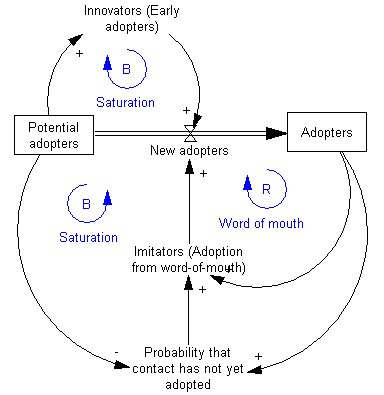
System Dynamics. A field often attributed to Jay Forrester at MIT (Sloan School). Characterized by largely graphical language for describing causal relationships.

By <a href="//commons.wikimedia.org/wiki/User:Patrhoue" title="User:Patrhoue">Patrhoue</a> - Own work, CC BY-SA 3.0, Link

3.12.3.1 Stock Diagrams¶

By The original uploader was <a href="https://en.wikipedia.org/wiki/User:Apdevries" class="extiw" title="wikipedia:User:Apdevries">Apdevries</a> at <a href="https://en.wikipedia.org/wiki/" class="extiw" title="wikipedia:">English Wikipedia</a>. - Transferred from <a class="external text" href="https://en.wikipedia.org">en.wikipedia</a> to Commons., CC BY-SA 3.0, Link

3.12.3.2 Causal Loops (Positive and Negative, Feedforward and Feedback)¶

By The original uploader was <a href="https://en.wikipedia.org/wiki/User:Apdevries" class="extiw" title="wikipedia:User:Apdevries">Apdevries</a> at <a href="https://en.wikipedia.org/wiki/" class="extiw" title="wikipedia:">English Wikipedia</a>. - Transferred from <a class="external text" href="https://en.wikipedia.org">en.wikipedia</a> to Commons., CC BY-SA 3.0, Link

3.12.3.3 AnyLogic¶

Download and install the Personal Learning Edition (https://www.anylogic.com/downloads/)
Download "AnyLogic in Three Days: Modeling and Simulation Textbook" (https://www.anylogic.com/resources/books/free-simulation-book-and-modeling-tutorials/)

< 3.11 Batch Chemical Process | Contents | 7.0 Risk and Diversification >