This notebook contains material from cbe30338-2021; content is available on Github.
In this lab you will:
These exercises are designed to reinforce concepts covered in the lecture component of the course, and to provide hands-on experience with the implementation of advanced PI control.
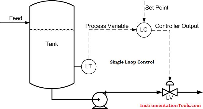
Cascade control is a means of coordinating individual controllers to incorporate additional sensors into the regulation of key control variables. To understand how this can work, consider a simple level control system

What are some typical disturbances?
The controller may do a good job with changes in feed flow rate, but what about changes in downstream pressure? Can we do better?

There is a nomenclature:
The job of the secondary flow controller is to maintain a desired flowrate. If it does its job then changes in flow due to downstream pressure, viscosity, or pump performance will be minimized before they substantially change in the tank level. The job of the primary level controller is to set the desired flowrate. It does this by providing a setpoint for operation of the inner loop.
This coordination of primary and secondary level controlers (or outer and inner controllers) uses multiple measurements (level and flow) to accomplish a single control objective (maintain constant level). The result is a faster response to disturbances and improved regulatory control.
This is a challenging lab assignment. Consequently, there will be no other homework assignment for the coming week. (Anything you would do there will covered in the course of this assignment.) To make the most efficient use of your time:
Get started right away. Open office hours on Monday will be extended as long as necessary to answer questions. I will only have limited availability later in the week.
Do the experiments in simulation mode to get started. Once you have things working in simulation, you will be able to perform the required experiments more quickly.
Use separate notebooks for the two exercises.
To avoid wasted time with accidental overwrites, manually rename any data files that you create. Data is precious.
You may work in groups of 2 to get your code working. Each student, however, must perform and submit the results of their own experiments.
The first taks is to implement PI control for temperature T2 using heater Q1. This is possible because of the significant heat transfer between the two heaters. The resulting control configuration is shown in the following diagram.

To complete this task:
To acheive the largest response, set lab.P1 = 255 for all subsequent experiments. You will use heater Q2 to introduce disturbances, so you can set lab.P2 = 50 for all experiments.
Choose a sample time 2 seconds or longer for all subsequent experiments.
Perform a step test measuring the response of temperature T2 to a step change in heater input Q1. The step input in Q1 should be limited to no more than 50% to avoid potential melting of the thermal paste in heater 1. Choose a sufficiently long time for the experiment so that you can accurately determine the steady state response. Save your data in a data file. You may wish to manually rename the data file to avoid accidently overwriting the file in subsequent experiments.
From the step test, fit a first order plus dead time (FOPDT) model. Report the parameters $K$ (steady-state gain), $T$ (time constant), and $\tau$ (time delay). Present a plot comparing your model fit to the measured data.
Use the Astrom and Murray tuning rules (see Notebook 3.5) to estimate values for the PI control parameters $K_P$ and $K_I$.
Implement an antiwindup version of PI control using the parameter values determined above. Test the performance of the controller in acheiving a setpoint of 30 deg C for temperature T2, and maintaining the setpoint following a disturbance where Q2 is set to 20% at t = 300 seconds.
For this task you will implement cascade control to regulate T2 to a setpoint using measuremnts of both T1 and T2, and compare the performance to the results you obtained in the first exercise. The control configuration is shown in the following diagram.

To complete this task:
In Lab Assignment 3 you implemented PI control for temperature T1 using heater Q1. This corresponds to the 'inner controller' shown in the diagram above. Update your implementation to incorporate antiwindup.
Verify performance of the inner controller to a step change in setpoint. You're looking for a step response with minimal or no overshoot of the setpoint. Estimate the time constant and dead time to a step change in setpoint. (Note that gain is not mentioned. Do you know what the gain will be before doing the experiment?)
Using empirical tuning rules, estimate proportional and integral gains for outer PI controller.
For the cascade control loop, perform the same testing as you did for the first exercise. Does cascade control improve closed response with respect to setpoint tracking? With respect to disturbance rejection. Explain what you see.