3.3 Linear Approximation of a Multivariable Model¶

3.3.1 Multivariable Systems¶

Most process models consist of more than a single state and a single input. Techniques for linearization extend naturally to multivariable systems. The most convenient mathematical tools involve some linear algebra.

3.3.1.1 Example: Gravity Drained Tanks¶

Here we develop a linear approximation to a process model for a system consisting of coupled gravity-drained tanks.

Gravity Drained Tanks

3.3.1.1.1 Model¶

\begin{eqnarray*} A_{1}\frac{dh_{1}}{dt} & = & q_{in}-C_{1}\sqrt{h_{1}}\\ A_{2}\frac{dh_{2}}{dt} & = & q_{d}+C_{1}\sqrt{h_{1}}-C_{2}\sqrt{h_{2}} \end{eqnarray*}

3.3.1.1.2 Nominal Inputs¶

\begin{eqnarray*} \bar{q}_{in} & = & \bar{q}_{in}\\ \bar{q}_{d} & = & 0 \end{eqnarray*}

3.3.1.1.3 Steady State for nominal input¶

\begin{eqnarray*} \bar{h}_{1} & = & \frac{\bar{q}_{in}^{2}}{C_{1}^{2}}\\ \bar{h}_{2} & = & \frac{\bar{q}_{in}^{2}}{C_{2}^{2}} \end{eqnarray*}

3.3.1.1.4 Deviation Variables¶

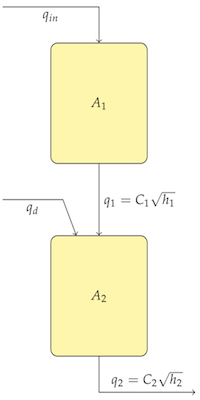
States

\begin{eqnarray*} x_{1} & = & h_{1}-\bar{h}_{1}\\ x_{2} & = & h_{2}-\bar{h}_{2} \end{eqnarray*}

Control input $$u=q_{in}-\bar{q}_{in}$$

Disturbance input $$d=q_{d}-\bar{q}_{d}$$

Measured output $$y=h_{2}-\bar{h}_{2}$$

3.3.1.1.5 Linearization¶

\begin{eqnarray*} \frac{dh_{1}}{dt} & = & \frac{1}{A_{1}}\left(q_{in}-C_{1}\sqrt{h_{1}}\right)=f_{1}(h_{1},h_{2},q_{in},q_{d})\\ \frac{dh_{2}}{dt} & = & \frac{1}{A_{2}}\left(q_{d}+C_{1}\sqrt{h_{1}}-C_{2}\sqrt{h_{2}}\right)=f_{2}(h_{1},h_{2},q_{in},q_{d}) \end{eqnarray*}

Taylor series expansion for the first tank

\begin{eqnarray*} \frac{dx_{1}}{dt} & = & f_{1}(\bar{h}_{1}+x_{1},\bar{h}_{2}+x_{2},\bar{q}_{in}+u,\bar{q}_{d}+d)\\ & \approx & \underbrace{f_{1}(\bar{h}_{1},\bar{h}_{2},\bar{q}_{in})}_{0}+\left.\frac{\partial f_{1}}{\partial h_{1}}\right|_{SS}x_{1}+\left.\frac{\partial f_{1}}{\partial h_{2}}\right|_{SS}x_{2}+\left.\frac{\partial f_{1}}{\partial q_{in}}\right|_{SS}u+\left.\frac{\partial f_{1}}{\partial q_{d}}\right|_{SS}d\\ & \approx & \left(-\frac{C_{1}}{2A_{1}\sqrt{\bar{h}_{1}}}\right)x_{1}+\left(0\right)x_{2}+\left(\frac{1}{A_{1}}\right)u+\left(0\right)d\\ & \approx & \left(-\frac{C_{1}^{2}}{2A_{1}\bar{q}_{in}}\right)x_{1}+\left(\frac{1}{A_{1}}\right)u \end{eqnarray*}

Taylor series expansion for the second tank

\begin{eqnarray*} \frac{dx_{2}}{dt} & = & f_{2}(\bar{h}_{1}+x_{1},\bar{h}_{2}+x_{2},\bar{q}_{in}+u,\bar{q}_{d}+d)\\ & \approx & \underbrace{f_{2}(\bar{h}_{1},\bar{h}_{2},\bar{q}_{in})}_{0}+\left.\frac{\partial f_{2}}{\partial h_{1}}\right|_{SS}x_{1}+\left.\frac{\partial f_{2}}{\partial h_{2}}\right|_{SS}x_{2}+\left.\frac{\partial f_{2}}{\partial q_{in}}\right|_{SS}u+\left.\frac{\partial f_{2}}{\partial q_{d}}\right|_{SS}d\\ & \approx & \left(\frac{C_{1}}{2A_{2}\sqrt{\bar{h}_{1}}}\right)x_{1}+\left(-\frac{C_{2}}{2A_{2}\sqrt{\bar{h}_{2}}}\right)x_{2}+\left(0\right)u+\left(\frac{1}{A_{2}}\right)d\\ & \approx & \left(\frac{C_{1}^{2}}{2A_{2}\bar{q}_{in}}\right)x_{1}+\left(-\frac{C_{2}^{2}}{2A_{2}\bar{q}_{in}}\right)x_{2}+\left(\frac{1}{A_{2}}\right)d \end{eqnarray*}

Measured outputs

\begin{eqnarray*} y & = & h_{2}-\bar{h}_{2}\\ & = & x_{2} \end{eqnarray*}

3.3.1.1.6 Summary of the linear model using matrix/vector notation¶

\begin{eqnarray*} \frac{d}{dt}\left[\begin{array}{c} x_{1}\\ x_{2} \end{array}\right] & = & \left[\begin{array}{cc} -\frac{C_{1}^{2}}{2A_{1}\bar{q}_{in}} & 0\\ \frac{C_{1}^{2}}{2A_{2}\bar{q}_{in}} & -\frac{C_{2}^{2}}{2A_{2}\bar{q}_{in}} \end{array}\right]\left[\begin{array}{c} x_{1}\\ x_{2} \end{array}\right]+\left[\begin{array}{c} \frac{1}{A_{1}}\\ 0 \end{array}\right]u+\left[\begin{array}{c} 0\\ \frac{1}{A_{2}} \end{array}\right]d\\ y & = & \left[\begin{array}{cc} 0 & 1\end{array}\right]\left[\begin{array}{c} x_{1}\\ x_{2} \end{array}\right]+\left[\begin{array}{c} 0\end{array}\right]u+\left[\begin{array}{c} 0\end{array}\right]d \end{eqnarray*}

3.3.2 Exercises¶

3.3.2.1 First Order Reaction in a CSTR¶

A first-order reaction

$$A\longrightarrow\mbox{Products}$$

takes place in an isothermal CSTR with constant volume $V$, volumetric flowrate in and out the same value $q$, reaction rate constant $k$, and feed concentration $c_{AF}$.

Write the material balance equation for this system as a first-order ordinary differential equation.
Algebraically determine the steady-state solution to this equation.
For what values of $q$, $k$, $V$, and $c_{AF}$ is this stable?
For a particular reaction $k$ = 2 1/min. We run this reaction in a vessel of volume $V$ =10 liters, volumetric flowrate $q$ = 50 liters/min. The desired exit concentrationof $A$ is $0.1$ gmol/liter. Assume that we can manipulate $c_{AF}$, the concentration of $A$ entering the CSTR, with proportional control, in order to control the concentration of $A$ exiting the reactor. Substitute the appropriate control law into the mathematical model and rearrange it to get a model of the same form as part (a).
Determine the steady-state solution to this equation. If we set $K_{c}=100$, what is the absolute value of the offset between the exit concentration of $A$ and the desired exit concentration of $A$?

3.3.2.2 Two Gravity Drained Tanks in Series¶

Consider the two-tank model. Assuming the tanks are identical, and using the same parameter values as used for the single gravity-drained tank, compute values for all coefficients appearing in the multivariable linear model. Is the system stable? What makes you think so?

3.3.2.3 Isothermal CSTR with second-order reaction¶

Consider an isothermal CSTR with a single reaction $$A\longrightarrow\mbox{Products}$$ whose reaction rate is second-order. Assume constant volume, $V$, and density, $\rho$, and a time-dependent volumetric flow rate $q(t)$. The input to the reactor has concentration $c_{A,in}$.

Write the modeling equation for this system.
Assume that the state variable is the concentration of $A$ in the output, $c_{A}$, and the flow rate $q$ is an input variable. There is a steady-state operating point corresponding to $q=1$ L/min. Other parameters are $k=1$ L/mol/min, $V=2$ L, $c_{A,in}=2$ mol/L. Find the linearized model for $\frac{dc'_{A}}{dt}$ valid in the neighborhood of this steady state.

< 3.2 Linear Approximation of a Process Model | Contents | Tag Index | 3.4 Fitting First Order plus Time Delay to Step Response >