2.3 Campus Re-opening Model¶

Following Paltiel, et al. (2020).

Paltiel2020-figure-e1

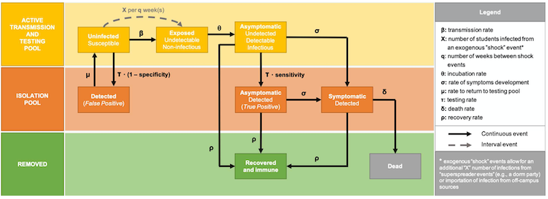
(Figure e1 from Paltiel, et al., 2020)

2.3.1 Active transmission and testing pool.¶

This pool consists of individuals in the campus population subject to testing and the transmission of virus.

$U$ uninfected, susceptible individuals
$E$ exposed, asymptomatic, non-infectious
$A$ infected, asymptomatic

\begin{align*} \frac{dU}{dt} & = -\beta U \frac{A}{U + E + A} - \tau (1-S_p) U + \mu F_p - x(t) \\ \frac{dE}{dt} & = \beta U \frac{A}{U + E + A} - \theta E + x(t) \\ \frac{dA}{dt} & = \theta E - (\sigma + \rho + \tau S_e)A \end{align*}

2.3.2 Isolation pool¶

$S$ infected, symptomatic with a true positive test result.
$T_p$ infected, asymptomatic with a true positive test result
$F_p$ uninfected with a false positive result.

\begin{align*} \frac{dF_p}{dt} & = -\mu F_p + \tau(1-S_p) U \\ \frac{dT_p}{dt} & = -(\sigma + \rho) T_p + \tau S_e A\\ \frac{dS}{dt} & = -(\rho + \delta)S + \sigma (T_p + A) \end{align*}

2.3.3 Removed pool¶

$R$ recovered. These individuals assumed to be immune for the remainder of the simulation, and not returned to the campus population.
$D$ dead.

\begin{align*} \frac{dR}{dt} & = \rho (T_p + A + S)\\\ \frac{dD}{dt} & = \delta S \end{align*}

2.3.4 Parameter estimates¶

Given:

$\rho$ recovery rate
$R_t$ basic reproductive number for asymptomatic transmission
$p_{si}$ probability that an infected individual will become symptomatic.

2.3.4.1 Odds of becoming symptomatic if infected¶

Based on the compartmental relationships and rates, the probability of symptom development for infected individuals is given by

$$p_{si} = \frac{\sigma}{\sigma + \rho}$$

Inverting this relationship

$$\sigma = \frac{p_{si}}{1 - p_{si}}\rho$$

where $\frac{p_{si}}{1 - p_{si}}$ is the 'odds' that an infected individual becomes symptomatic.

2.3.4.2 Effective reproductive number with isolation of symptomatic individuals¶

For an initially uninfected population with no testing regime, where transmission is solely due to non-isolated, asymptomatic individuals, the effective reproductive number is

$$R_t = \frac{\beta}{\sigma + \rho}$$

Expressed in terms of recovery rate and probability of becoming symptomatic

$$R_t = \frac{\beta}{\rho}(1 - p_{si})$$

2.3.4.3 Testing threshold¶

With a testing regime, for effective herd immunity requires

$$\beta \leq \sigma + \rho + \tau S_e $$

where $\tau$ is the testing rate and $S_e$ is the test sensitivity. With some manipulation using the above relationships, the testing treshhold becomes

$$\tau S_e \geq \frac{(R_t - 1) \rho}{1 - p_{si}}$$

or

$$\frac{1}{\tau} \leq S_e \left(\frac{1 - p_{si}}{R_t - 1}\right)\frac{1}{\rho} $$

2.3.4.4 Parameter values¶

parameter	value
$p_{si}$	0.3
$R_t$	[1.5, 2.5, 3.5]
$\frac{1}{\rho}$	14 d
$S_e$	0.7

t

import numpy as np
import matplotlib.pyplot as plt
import seaborn as sns

Rt = np.linspace(1.5, 4.0)
Se = 0.7
rho = 1/14.0
psi = 0.3

tau = (Rt - 1)*rho/(1 - psi)
plt.plot(Rt, 1.0/tau)

plt.xlabel('$R_t$: effective reproduction number for exclusively asymptomatic transmission')
plt.ylabel('testing frequency / days')
plt.grid(True)

import numpy as np
from scipy.integrate import solve_ivp
import matplotlib.pyplot as plt
import seaborn as sns

# time horizon in days
d = 15 * 7   

# disease dynamics
Rt = 4.0
theta = 1/3.0       # 1/incubation time in days
rho = 1.0/14.0      # 1/time to recovery in days
mu = 1.0/1.0        # 1/time to false-postive return in days
p_si = 0.20        # probability of symptoms given infection
p_fs = 0.0005      # probability of fataility given symptoms

sigma = rho * p_si / (1 - p_si)      # rate of symptom development
beta = (sigma + rho)*Rt
delta = rho * (p_fs/p_si) / (1 - (p_fs/p_si))

# testing protocols
Sp = 0.98       # test specificity
Se = 0.70       # test sensitivity
tau = 1000        # testing period

# population parameters
x = 10.0        # weekly exogeneous infections
y = 10.0
IC = [8200-y, 0, y, 0, 0, 0, 0, 0]

# SEIR model differential equations.
def deriv(t, X):
    U, E, A, S, Tp, Fp, R, D = X
    exog = x*((t + 1) % 7 < 1)
    dU = -beta*U*A/(U + E + A + R) - (1 - Sp)*U/tau + mu*Fp - exog
    dE = beta*U*A/(U + E + A + R) - theta*E + exog
    dA = theta*E - (sigma + rho + Se/tau)*A
    dS = -(rho + delta)*S + sigma*(Tp + A)
    dTp = -(sigma + rho)*Tp + Se*A/tau
    dFp = -mu*Fp + (1 - Sp)*U/tau
    dR = rho*(Tp + S + A)
    dD = delta*S
    return np.array([dU, dE, dA, dS, dTp, dFp, dR, dD,])

t = np.linspace(0, d, 10*d + 1)
soln = solve_ivp(deriv, [0, max(t)], IC, t_eval = t, atol=1e-8, rtol=1e-8)
U, E, A, S, Tp, Fp, R, D = soln.y

fix, ax = plt.subplots(3, 1, figsize=(12, 8))
ax[0].stackplot(t, U, E, A, R)
ax[0].set_ylim(0, sum(IC))
ax[0].set_title('Active Transmission and Testing Pool')

ax[1].stackplot(t, S, Tp, Fp)
ax[1].legend(['Symptomatic', 'False Positive', 'True Positive'], loc="upper left")
ax[1].set_title('Isolation Pool')

ax[2].stackplot(t, D)
ax[2].set_title('Removed Pool')
ax[2].legend(['Recovered', 'Dead'], loc="upper left")

for a in ax:
    a.set_xlim(0, d)

plt.tight_layout()

< 2.2 Campus SEIR Modeling | Contents | 2.4 Linear Analysis of Campus Reopening >