1.4. Case Study: Analysis of a Double Pipe Heat Exchanger¶

A stalwart of undergraduate chemical engineering laboratories is study of a double-pipe heat exchanger in counter-current flow. In this case, a student group collected multiple measurements of flow and temperature data from a heat exchanger with sensors configured as shown in the following diagram. (Note: The diagram shows co-current flow. The data was collected with the valves configured for counter-current flow of the hot stream.)

Source: Gunt WL315C Product Description

1.4.1. Reading Data¶

The raw data was copied to a new sheet in the same Google Sheets file, edited to conform with Tidy Data, and a link created using the procedures outlined above for reading data from Google Sheets. The data is read in the following cell.

hx = pd.read_csv("https://docs.google.com/spreadsheets/d/e/2PACX-1vSNUCEFMaGZ-y18p-AnDoImEeenMLbRxXBABwFNeP8I3xiUejolPJx-kr4aUywD0szRel81Kftr8J0R/pub?gid=865146464&single=true&output=csv")
hx.head()

	Flow Rate H	Flow Rate C	Trial #	Hot Flow (L/hr)	Cold Flow (L/hr)	Time	H Outlet	H Inlet	C Inlet	C Outlet
0	H	H	1	651	798	32:08.1	37.3	56.4	15.5	30.8
1	H	H	1	651	798	32:07.8	37.2	56.3	15.4	30.8
2	H	H	1	651	798	32:07.6	37.2	56.3	15.4	30.8
3	H	M	2	650	512	29:13.0	41.4	56.4	15.6	34.7
4	H	M	2	650	512	29:12.3	41.4	56.4	15.6	34.7

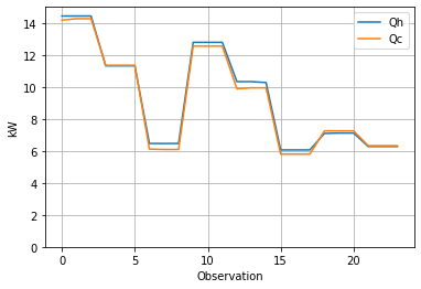
1.4.2. Energy Balances¶

The first step in this analysis is to verify the energy balance.

\[\begin{split} \begin{align*} Q_h & = \dot{q}_h \rho C_p (T_{h,in} - T_{h,out}) \\ Q_c & = \dot{q}_c \rho C_p (T_{c,out} - T_{c, in}) \end{align*} \end{split}\]

The next cell creates two new calculated variables in the dataframe for \(Q_h\) and \(Q_c\), and uses the pandas plotting facility to visualize the results. This calculation takes advantage of the “one variable per column” rule of Tidy Data which enables calculations for all observations to be done in a single line of code.

# heat capacity of water 
rho = 1.00                # kg / liter
Cp = 4.18                 # kJ/ kg / deg C

# heat balances
hx["Qh"] = rho * Cp * hx["Hot Flow (L/hr)"] * (hx["H Inlet"] - hx["H Outlet"]) / 3600
hx["Qc"] = rho * Cp * hx["Cold Flow (L/hr)"] * (hx["C Outlet"] - hx["C Inlet"]) / 3600
hx["Loss (%)"] = 100 * (1 - hx["Qc"]/hx["Qh"])

# plot
display(hx[["Qh", "Qc", "Loss (%)"]].style.format(precision=2))
hx.plot(y = ["Qh", "Qc"], ylim = (0, 15), grid=True, xlabel="Observation", ylabel="kW")

	Qh	Qc	Loss (%)
0	14.44	14.18	1.81
1	14.44	14.27	1.17
2	14.44	14.27	1.17
3	11.32	11.35	-0.30
4	11.32	11.35	-0.30
5	11.32	11.35	-0.30
6	6.46	6.11	5.41
7	6.46	6.09	5.77
8	6.46	6.09	5.77
9	12.79	12.55	1.85
10	12.79	12.55	1.85
11	12.79	12.55	1.85
12	10.33	9.89	4.32
13	10.33	9.95	3.76
14	10.28	9.95	3.21
15	6.06	5.80	4.33
16	6.06	5.80	4.33
17	6.06	5.80	4.33
18	7.09	7.25	-2.27
19	7.12	7.25	-1.93
20	7.12	7.25	-1.93
21	6.28	6.33	-0.81
22	6.28	6.33	-0.81
23	6.28	6.33	-0.81

<AxesSubplot:xlabel='Observation', ylabel='kW'>

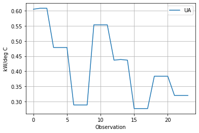
1.4.3. Overall Heat Transfer Coefficient \(UA\)¶

The performance of a counter-current heat exchanger is given the relationship

\[Q = U A \Delta T_{lm} \]

where \(\Delta T_{lm}\) is the log-mean temperature given by

\[\begin{split} \begin{align*} \Delta T_0 & = T_{h, out} - T_{c, in} \\ \Delta T_1 & = T_{h, in} - T_{c, out} \\ \\ \Delta T_{lm} & = \frac{\Delta T_1 - \Delta T_0}{\ln\frac{\Delta T_1}{\Delta T_0}} \end{align*} \end{split}\]

dT0 = hx["H Outlet"] - hx["C Inlet"]
dT1 = hx["H Inlet"] - hx["C Outlet"]
hx["LMTD"] = (dT1 - dT0) / np.log(dT1/dT0)

Q = (hx.Qh + hx.Qc)/2
hx["UA"] =  Q/hx.LMTD

hx.plot(y="UA", xlabel="Observation", ylabel="kW/deg C", grid=True)

<AxesSubplot:xlabel='Observation', ylabel='kW/deg C'>

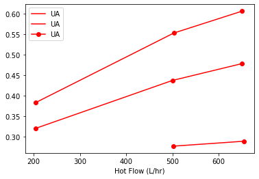
1.4.4. How does \(UA\) depend on flowrates?¶

The data clearly demonstrate that the heat transfer coefficient in the double pipe heat exchanger depends on flowrates of both the cold and hot liquid streams. We can see this by inspecting the data.

hx[["Flow Rate H", "Flow Rate C", "Hot Flow (L/hr)", "Cold Flow (L/hr)", "UA"]]

	Flow Rate H	Flow Rate C	Hot Flow (L/hr)	Cold Flow (L/hr)	UA
0	H	H	651	798	0.604966
1	H	H	651	798	0.608145
2	H	H	651	798	0.608145
3	H	M	650	512	0.478571
4	H	M	650	512	0.478571
5	H	M	650	512	0.478571
6	H	L	655	201	0.288997
7	H	L	655	201	0.288976
8	H	L	655	201	0.288976
9	M	H	503	795	0.553374
10	M	H	503	795	0.553374
11	M	H	503	795	0.553374
12	M	M	500	498	0.436787
13	M	M	500	498	0.438975
14	M	M	500	498	0.436765
15	M	L	502	199	0.276936
16	M	L	502	199	0.276936
17	M	L	502	199	0.276936
18	L	H	205	801	0.383826
19	L	H	205	801	0.383744
20	L	H	205	801	0.383744
21	L	M	204	500	0.320247
22	L	M	204	500	0.320247
23	L	M	204	500	0.320247

The replicated measurements provide an opportunity to compute averages. Here we use the pandas .groupby() function to group observations and compute means. The data will be used to plot results, so we’ll save the results of these calculations as a new dataframe for reuse.

sx = hx.groupby(["Flow Rate H", "Flow Rate C"]).mean()[["Hot Flow (L/hr)", "Cold Flow (L/hr)", "UA"]]
sx

		Hot Flow (L/hr)	Cold Flow (L/hr)	UA
Flow Rate H	Flow Rate C
H	H	651.0	798.0	0.607085
	L	655.0	201.0	0.288983
	M	650.0	512.0	0.478571
L	H	205.0	801.0	0.383771
L	M	204.0	500.0	0.320247
M	H	503.0	795.0	0.553374
	L	502.0	199.0	0.276936
	M	500.0	498.0	0.437509

import matplotlib.pyplot as plt

fig, ax = plt.subplots(1, 1)
sx.sort_values("Cold Flow (L/hr)").groupby("Flow Rate H").plot(x = "Cold Flow (L/hr)", y = "UA", 
                                                               style={"UA": 'ro-'}, ax=ax)

Flow Rate H
H    AxesSubplot(0.125,0.125;0.775x0.755)
L    AxesSubplot(0.125,0.125;0.775x0.755)
M    AxesSubplot(0.125,0.125;0.775x0.755)
dtype: object

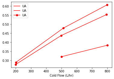
fig, ax = plt.subplots(1, 1)
sx.sort_values("Hot Flow (L/hr)").groupby("Flow Rate C").plot(x = "Hot Flow (L/hr)", y = "UA", 
                                                               style={"UA": 'ro-'}, ax=ax)

Flow Rate C
H    AxesSubplot(0.125,0.125;0.775x0.755)
L    AxesSubplot(0.125,0.125;0.775x0.755)
M    AxesSubplot(0.125,0.125;0.775x0.755)
dtype: object

1.4.5. Fitting a Model for \(UA\)¶

For a series of transport mechanisms, the overall heat transfer coefficient

\[\frac{1}{UA} = \frac{1}{U_hA} + \frac{1}{U_{tubeA}} + \frac{1}{U_cA}\]

\(U_{tube}A\) is a constant for this experiment. \(U_h\)A and \(U_c\)A varying with flowrate and proporitonal to dimensionless Nusselt number. The hot and cold liquid flows in the double pipe heat exchanger are well within the range for fully developed turbulent flow. Under these conditions for flows inside closed tubes, the Dittus-Boelter equation provides an explicit expression for Nusselt number

\[Nu = C \cdot Re ^{4/5} Pr ^ n\]

where \(C\) is a constant, \(Re\) is the Reynold’s number that is proportional to flowrate, and \(Pr\) is the Prandtl number determined by fluid properties.

Experimentally, consider a set of values for \(UA\) determined by varying \(\dot{m}_h\) and \(\dot{m}_c\) over range of values. Because Reynold’s number is proportional to flowrate, we can propose a model

\[\frac{1}{UA} = R = R_{t} + r_h \dot{q}_h^{-0.8} + r_c \dot{q}_h^{-0.8}\]

This suggests a linear regression for \(R = \frac{1}{UA}\) in terms of \(X_h = \dot{q}_h^{-0.8}\) and \(X_c = \dot{q}_c^{-0.8}\).

Enhancement: Convert to Skikit-learn

The following model fit should be converted to Scikit-learn to enable use of ML tools to the model building process.

hx["R"] = 1.0/hx["UA"]
hx["Xh"] = hx["Hot Flow (L/hr)"]**(-0.8)
hx["Xc"] = hx["Cold Flow (L/hr)"]**(-0.8)

import statsmodels.formula.api as sm

result = sm.ols(formula="R ~ Xh + Xc", data = hx).fit()
print(result.params)
print(result.summary())

Intercept      0.141716
Xh           115.292199
Xc           186.346764
dtype: float64
                            OLS Regression Results                            
==============================================================================
Dep. Variable:                      R   R-squared:                       0.997
Model:                            OLS   Adj. R-squared:                  0.997
Method:                 Least Squares   F-statistic:                     3711.
Date:                Tue, 01 Feb 2022   Prob (F-statistic):           1.70e-27
Time:                        08:53:59   Log-Likelihood:                 44.929
No. Observations:                  24   AIC:                            -83.86
Df Residuals:                      21   BIC:                            -80.32
Df Model:                           2                                         
Covariance Type:            nonrobust                                         
==============================================================================
                 coef    std err          t      P>|t|      [0.025      0.975]
------------------------------------------------------------------------------
Intercept      0.1417      0.032      4.425      0.000       0.075       0.208
Xh           115.2922      2.465     46.762      0.000     110.165     120.419
Xc           186.3468      2.233     83.445      0.000     181.703     190.991
==============================================================================
Omnibus:                        9.087   Durbin-Watson:                   0.894
Prob(Omnibus):                  0.011   Jarque-Bera (JB):                2.268
Skew:                           0.227   Prob(JB):                        0.322
Kurtosis:                       1.564   Cond. No.                         334.
==============================================================================

Notes:
[1] Standard Errors assume that the covariance matrix of the errors is correctly specified.

hx["Rh"] = 115.3 * hx["Xh"]
hx["Rc"] = 186.3 * hx["Xc"]
hx["Rt"] = 0.142

hx["R_pred"] = hx["Rt"] + hx["Rh"] + hx["Rc"]
hx[["R", "R_pred", "Rt", "Rh", "Rc"]]

	R	R_pred	Rt	Rh	Rc
0	1.652986	1.677494	0.142	0.647090	0.888404
1	1.644344	1.677494	0.142	0.647090	0.888404
2	1.644344	1.677494	0.142	0.647090	0.888404
3	2.089553	2.056945	0.142	0.647886	1.267059
4	2.089553	2.056945	0.142	0.647886	1.267059
5	2.089553	2.056945	0.142	0.647886	1.267059
6	3.460242	3.462974	0.142	0.643926	2.677047
7	3.460489	3.462974	0.142	0.643926	2.677047
8	3.460489	3.462974	0.142	0.643926	2.677047
9	1.807095	1.828466	0.142	0.795380	0.891085
10	1.807095	1.828466	0.142	0.795380	0.891085
11	1.807095	1.828466	0.142	0.795380	0.891085
12	2.289447	2.236672	0.142	0.799196	1.295476
13	2.278034	2.236672	0.142	0.799196	1.295476
14	2.289559	2.236672	0.142	0.799196	1.295476
15	3.610936	3.637197	0.142	0.796648	2.698550
16	3.610936	3.637197	0.142	0.796648	2.698550
17	3.610936	3.637197	0.142	0.796648	2.698550
18	2.605346	2.658637	0.142	1.630896	0.885741
19	2.605903	2.658637	0.142	1.630896	0.885741
20	2.605903	2.658637	0.142	1.630896	0.885741
21	3.122589	3.070617	0.142	1.637288	1.291329
22	3.122589	3.070617	0.142	1.637288	1.291329
23	3.122589	3.070617	0.142	1.637288	1.291329

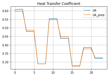
1.4.6. Comparison of Model to Experimental Data¶

hx["UA_pred"] = 1/hx["R_pred"]
hx.plot(y = ["UA", "UA_pred"], grid=True, title="Heat Transfer Coefficient")

<AxesSubplot:title={'center':'Heat Transfer Coefficient'}>

CBE 31358 Laboratory I

Case Study: Analysis of a Double Pipe Heat Exchanger

Contents