Measuring Return
Contents
Measuring Return#
Imports#
The pandas_datareader library provides convenient access to financial data. The library requires separate installation by executing the command
pip install pandas-datareader
in a terminal window, or executign
!pip install pandas-datareader --upgrade
in a Jupyter notebook cell.
!pip install pandas-datareader --upgrade
Looking in indexes: https://pypi.org/simple, https://us-python.pkg.dev/colab-wheels/public/simple/
Requirement already satisfied: pandas-datareader in /usr/local/lib/python3.7/dist-packages (0.10.0)
Requirement already satisfied: pandas>=0.23 in /usr/local/lib/python3.7/dist-packages (from pandas-datareader) (1.3.5)
Requirement already satisfied: requests>=2.19.0 in /usr/local/lib/python3.7/dist-packages (from pandas-datareader) (2.23.0)
Requirement already satisfied: lxml in /usr/local/lib/python3.7/dist-packages (from pandas-datareader) (4.9.1)
Requirement already satisfied: pytz>=2017.3 in /usr/local/lib/python3.7/dist-packages (from pandas>=0.23->pandas-datareader) (2022.6)
Requirement already satisfied: numpy>=1.17.3 in /usr/local/lib/python3.7/dist-packages (from pandas>=0.23->pandas-datareader) (1.21.6)
Requirement already satisfied: python-dateutil>=2.7.3 in /usr/local/lib/python3.7/dist-packages (from pandas>=0.23->pandas-datareader) (2.8.2)
Requirement already satisfied: six>=1.5 in /usr/local/lib/python3.7/dist-packages (from python-dateutil>=2.7.3->pandas>=0.23->pandas-datareader) (1.15.0)
Requirement already satisfied: idna<3,>=2.5 in /usr/local/lib/python3.7/dist-packages (from requests>=2.19.0->pandas-datareader) (2.10)
Requirement already satisfied: urllib3!=1.25.0,!=1.25.1,<1.26,>=1.21.1 in /usr/local/lib/python3.7/dist-packages (from requests>=2.19.0->pandas-datareader) (1.24.3)
Requirement already satisfied: chardet<4,>=3.0.2 in /usr/local/lib/python3.7/dist-packages (from requests>=2.19.0->pandas-datareader) (3.0.4)
Requirement already satisfied: certifi>=2017.4.17 in /usr/local/lib/python3.7/dist-packages (from requests>=2.19.0->pandas-datareader) (2022.9.24)
%matplotlib inline
import matplotlib.pyplot as plt
import numpy as np

import pandas as pd
import datetime
import pandas_datareader as pdr
The following function provides a convenient stock symbol lookup function.
Where to get Price Data#
Price data is available from a number of sources. Here we demonstrate the process of obtaining price data on financial goods from Yahoo Finance. Additional sources are documented here.
Yahoo Finance#
Yahoo Finance provides historical Open, High, Low, Close, and Volume date for quotes on traded securities. In addition, Yahoo Finance provides historical Adjusted Close price data that corrects for splits and dividend distributions. The Adjusted Close is a useful tool for computing the return on long-term investments.
The following cell demonstrates how to download historical Adjusted Close price for a selected security into a pandas DataFrame.
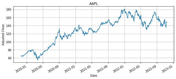
symbol = 'AAPL'

# end date is today
end = datetime.datetime.today().date()

# start date is three years prior
start = end-datetime.timedelta(3*365)

# get stock price data
S = pdr.data.DataReader(symbol, "yahoo", start, end)['Adj Close']

# plot data
plt.figure(figsize=(10,4))
S.plot(title=symbol, grid=True, ylabel="Adjusted Close")
<matplotlib.axes._subplots.AxesSubplot at 0x7f55bc75f250>
Quandl#
Quandl is a searchable source of time-series data on a wide range of commodities, financials, and many other economic and social indicators. Data from Quandl can be downloaded as files in various formats, or accessed directly using the Quandl API or software-specific package. Here we use demonstrate use of the Quandl Python package.
The first step is execute a system command to check that the Quandl package has been installed.
Here are examples of energy datasets. These were found by searching Quandl, then identifying the Quandl code used for accessing the dataset, a description, the name of the field containing the desired price information.
code = 'CHRIS/MCX_CL1'
description = 'NYMEX Crude Oil Futures, Continuous Contract #1 (CL1) (Front Month)'
field = 'Close'
end = datetime.datetime.today().date()
start = end - datetime.timedelta(5*365)

S = pdr.quandl.QuandlReader(code, start, end)

plt.figure(figsize=(10,4))
S.plot()
plt.title(description)
plt.ylabel('Price $/bbl')
plt.grid()
---------------------------------------------------------------------------
ValueError                                Traceback (most recent call last)
<ipython-input-16-e46d8d827ff0> in <module>
      2 start = end - datetime.timedelta(5*365)
      3
----> 4 S = pdr.quandl.QuandlReader(code, start, end)
      5
      6 plt.figure(figsize=(10,4))

/usr/local/lib/python3.7/dist-packages/pandas_datareader/quandl.py in __init__(self, symbols, start, end, retry_count, pause, session, chunksize, api_key)
     64         if not api_key or not isinstance(api_key, str):
     65             raise ValueError(
---> 66                 "The Quandl API key must be provided either "
     67                 "through the api_key variable or through the "
     68                 "environmental variable QUANDL_API_KEY."

ValueError: The Quandl API key must be provided either through the api_key variable or through the environmental variable QUANDL_API_KEY.
Returns#
The statistical properties of financial series are usually studied in terms of the change in prices. There are several reasons for this, key among them is that the changes can often be closely approximated as stationary random variables whereas prices are generally non-stationary sequences.
A common model is
so, recursively,
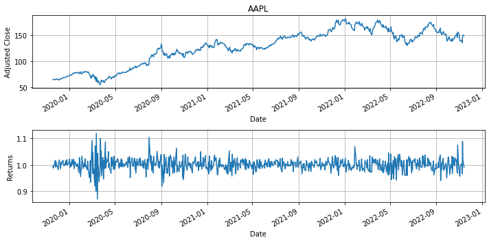
The gross return \(R_t\) is simply the ratio of the current price to the previous, i.e.,
\(R_t\) will typically be a number close to one in value, greater than one for an appreciating asset, or less than one for an asset with declining price.
symbol = 'AAPL'

# end date is today
end = datetime.datetime.today().date()

# start date is three years prior
start = end-datetime.timedelta(3*365)

# get stock price data
S = pdr.data.DataReader(symbol,"yahoo", start, end)['Adj Close']
R = S/S.shift(1)

# plot data
plt.figure(figsize=(10, 5))
plt.subplot(2,1,1)
S.plot(title=symbol, ylabel="Adjusted Close", grid=True)

plt.subplot(2, 1, 2)
R.plot(ylabel="Returns", grid=True)
plt.tight_layout()
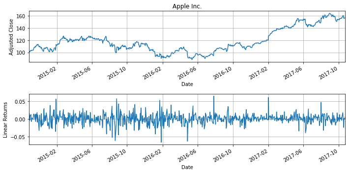
Linear fractional or Arithmetic Returns#
Perhaps the most common way of reporting returns is simply the fractional increase in value of an asset over a period, i.e.,
Obviously
symbol = 'AAPL'

# end date is today
end = datetime.datetime.today().date()

# start date is three years prior
start = end-datetime.timedelta(3*365)

# get stock price data
S = data.DataReader(symbol,"yahoo",start,end)['Adj Close']
rlin = S/S.shift(1) - 1

# plot data
plt.figure(figsize=(10,5))
plt.subplot(2,1,1)
S.plot(title=get_symbol(symbol))
plt.ylabel('Adjusted Close')
plt.grid()

plt.subplot(2,1,2)
rlin.plot()
plt.title('Linear Returns (daily)')
plt.grid()
plt.tight_layout()
Linear returns don’t tell the whole story.#
Suppose you put money in an asset that returns 10% interest in even numbered years, but loses 10% in odd numbered years. Is this a good investment for the long-haul?
If we look at mean linear return
\begin{align} \bar{r}^{lin} & = \frac{1}{T}\sum_{t=1}{T} r^{lin}_t \ & = \frac{1}{T} (0.1 - 0.1 + 0.1 - 0.1 + \cdots) \ & = 0 \end{align}
we would conclude this asset, on average, offers zero return. What does a simulation show?
S = 100
log = [[0,S]]
r = 0.10

for k in range(1,101):
    S = S + r*S
    r = -r
    log.append([k,S])

df = pd.DataFrame(log,columns = ['k','S'])
plt.plot(df['k'],df['S'])
plt.xlabel('Year')
plt.ylabel('Value')
Text(0, 0.5, 'Value')
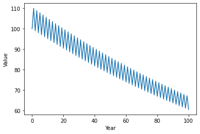
Despite an average linear return of zero, what we observe over time is an asset declining in price. The reason is pretty obvious — on average, the years in which the asset loses money have higher balances than years where the asset gains value. Consequently, the losses are somewhat greater than the gains which, over time, leads to a loss of value.
Here’s a real-world example of this phenomenon. For a three year period ending October 24, 2017, United States Steel (stock symbol ‘X’) offers an annualized linear return of 15.9%. Seems like a terrific investment opportunity, doesn’t it? Would you be surprised to learn that the actual value of the stock fell 18.3% over that three-year period period?
What we can conclude from these examples is that average linear return, by itself, does not provide us with the information needed for long-term investing.
symbol = 'X'

# end date is today
end = datetime.datetime(2017, 10, 24)

# start date is three years prior
start = end-datetime.timedelta(3*365)

# get stock price data
S = pdr.data.DataReader(symbol, "yahoo", start, end)['Adj Close']
rlin = S/S.shift(1) - 1

print('Three year return :', 100*(S[-1]-S[0])/S[0], '%')

# plot data
plt.figure(figsize=(10, 5))
plt.subplot(2, 1, 1)
S.plot(title=symbol, ylabel="Adjusted Close", grid=True)


plt.subplot(2, 1, 2)
rlin.plot(title=f'Mean Linear Returns (annualized) = {0:.2f}%'.format(100*252*rlin.mean()))
plt.grid()
plt.tight_layout()
Three year return : -18.38049353595533 %
---------------------------------------------------------------------------
NameError                                 Traceback (most recent call last)
<ipython-input-26-76ba57adfc98> in <module>
     16 plt.figure(figsize=(10,5))
     17 plt.subplot(2,1,1)
---> 18 S.plot(title=get_symbol(symbol))
     19 plt.ylabel('Adjusted Close')
     20 plt.grid()

NameError: name 'get_symbol' is not defined
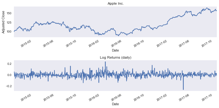
Compounded Log Returns#
Compounded, or log returns, are defined as
The log returns have a very useful compounding property for aggregating price changes across time
If the compounded returns are statistically independent and identically distributed, then this property provides a means to aggregate returns and develop statistical price projections.
symbol = 'AAPL'

# end date is today
end = datetime.datetime.today().date()

# start date is three years prior
start = end-datetime.timedelta(3*365)

# get stock price data
S = data.DataReader(symbol,"yahoo",start,end)['Adj Close']
rlog = np.log(S/S.shift(1))

# plot data
plt.figure(figsize=(10,5))
plt.subplot(2,1,1)
S.plot(title=get_symbol(symbol))
plt.ylabel('Adjusted Close')
plt.grid()

plt.subplot(2,1,2)
rlin.plot()
plt.title('Log Returns (daily)')
plt.grid()
plt.tight_layout()
Volatility Drag and the Relationship between Linear and Log Returns#
For long-term financial decision making, it’s important to understand the relationship between \(r_t^{log}\) and \(r_t^{lin}\). Algebraically, the relationships are simple.
The linear return \(r_t^{lin}\) is the fraction of value that is earned from an asset in a single period. It is a direct measure of earnings. The average value \(\bar{r}^{lin}\) over many periods this gives the average fractional earnings per period. If you care about consuming the earnings from an asset and not about growth in value, then \(\bar{r}^{lin}\) is the quantity of interest to you.
Log return \(r_t^{log}\) is the rate of growth in value of an asset over a single period. When averaged over many periods, \(\bar{r}^{log}\) measures the compounded rate of growth of value. If you care about the growth in value of an asset, then \(\bar{r}^{log}\) is the quantity of interest to you.
The compounded rate of growth \(r_t^{log}\) is generally smaller than average linear return \(\bar{r}^{lin}\) due to the effects of volatility. To see this, consider an asset that has a linear return of -50% in period 1, and +100% in period 2. The average linear return is would be +25%, but the compounded growth in value would be 0%.
A general formula for the relationship between \(\bar{r}^{log}\) and \(\bar{r}^{lin}\) is derived as follows:
For typical values \(\bar{r}^{lin}\) of and long horizons \(T\), this results in a formula
where \(\sigma^{lin}\) is the standard deviation of linear returns, more commonly called the volatility.
The difference \(- \frac{1}{2} \left(\sigma^{lin}\right)^2\) is the volatility drag imposed on the compounded growth in value of an asset due to volatility in linear returns. This can be significant and a source of confusion for many investors.
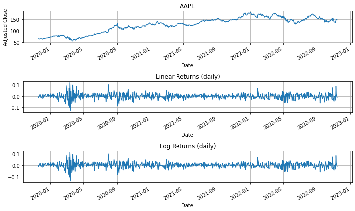
It’s indeed possible to have a positive average linear return, but negative compounded growth. To see this, consider a $100 investment which earns 20% on even-numbered years, and loses 18% on odd-numbered years. The average linear return is 1%, and the average log return is -0.81%.
symbol = 'AAPL'

# end date is today
end = datetime.datetime.today().date()

# start date is three years prior
start = end-datetime.timedelta(3*365)

# get stock price data
S = pdr.data.DataReader(symbol, "yahoo", start, end)['Adj Close']
rlin = (S - S.shift(1))/S.shift(1)
rlog = np.log(S/S.shift(1))

# plot data
plt.figure(figsize=(10,6))
plt.subplot(3,1,1)
S.plot(title=symbol)
plt.ylabel('Adjusted Close')
plt.grid()

plt.subplot(3,1,2)
rlin.plot()
plt.title('Linear Returns (daily)')
plt.grid()
plt.tight_layout()

plt.subplot(3,1,3)
rlog.plot()
plt.title('Log Returns (daily)')
plt.grid()
plt.tight_layout()
print("Mean Linear Return (rlin) = {0:.7f}".format(rlin.mean()))
print("Linear Volatility (sigma) = {0:.7f}".format(rlin.std()))
print("Volatility Drag -0.5*sigma**2 = {0:.7f}".format(-0.5*rlin.std()**2))
print("rlin - 0.5*vol = {0:.7f}\n".format(rlin.mean() - 0.5*rlin.std()**2))

print("Mean Log Return = {0:.7f}".format(rlog.mean()))
Mean Linear Return (rlin) = 0.0013522
Linear Volatility (sigma) = 0.0230372
Volatility Drag -0.5*sigma**2 = -0.0002654
rlin - 0.5*vol = 0.0010868

Mean Log Return = 0.0010867
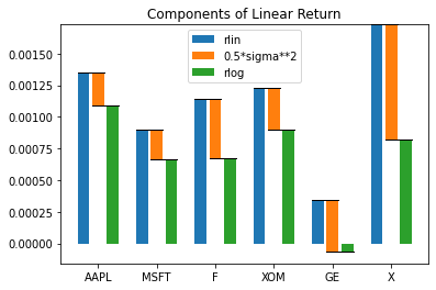
symbols = ['AAPL', 'MSFT', 'F', 'XOM', 'GE', 'X']

# end date is today
end = datetime.datetime.today().date()

# start date is three years prior
start = end - datetime.timedelta(3*365)

rlin = []
rlog = []
sigma = []

for symbol in symbols:

    # get stock price data
    S = pdr.data.DataReader(symbol, "yahoo", start, end)['Adj Close']
    r = (S - S.shift(1))/S.shift(1)
    rlin.append(r.mean())
    rlog.append((np.log(S/S.shift(1))).mean())
    sigma.append(r.std())
import seaborn as sns
N = len(symbols)
idx = np.arange(N)
width = 0.2

p0 = plt.bar(idx - 1.25*width, rlin, width)
p1 = plt.bar(idx, -0.5*np.array(sigma)**2, width, bottom=rlin)
p2 = plt.bar(idx + 1.25*width, rlog, width)

for k in range(0,N):
    plt.plot([k - 1.75*width, k + 0.5*width],[rlin[k],rlin[k]],'k',lw=1)
    plt.plot([k - 0.5*width, k + 1.75*width],[rlog[k],rlog[k]],'k',lw=1)

plt.xticks(idx,symbols)
plt.legend((p0[0],p1[0],p2[0]),('rlin','0.5*sigma**2','rlog'))
plt.title('Components of Linear Return')
Text(0.5, 1.0, 'Components of Linear Return')