Portfolio Optimization#

This Jupyter notebook demonstrates the formulation and solution of portfolio optimization problems.

Import libraries#

import matplotlib.pyplot as plt
import numpy as np
import random

# data wrangling libraries
import pandas_datareader.data as web
import pandas as pd
import datetime

Load Price Data#

Here we create several groups of possible trading symbols, and select one for study.

# Companies of the Dow Jones Industrial Average
djia = ['axp', 'aapl', 'amgn', 'ba', 'cat', 'crm', 'cvx', 'csco',  'dis', 'dow',
        'gs', 'hd', 'hon', 'ibm', 'intc', 'jnj', 'jpm', 'ko', 'mcd', 'mmm', 'mrk',
        'msft', 'nke', 'pg', 'trv', 'unh', 'vz', 'v', 'wba', 'wmt']

# Representative ETF's and ETN's from the energy sector
energy = ['uso', 'ung', 'tan', 'wndy', ]

# Standard indices
indices = ['^dji', '^gspc']

# pick one of these groups for study
symbols = djia[0:5]
#symbols = energy
print(symbols)

['axp', 'aapl', 'amgn', 'ba', 'cat']

Price data is retrieved using the Pandas DataReader function. The first price data set consists of historical data that will be used to design investment portfolios. The second set will be used for simulation and evaluation of resulting portfolios. The use of ‘out-of-sample’ data for evaluation is standard practice in these types of applications.

t2 = datetime.datetime.now()
t1 = t2 - datetime.timedelta(365)
t0 = t1 - datetime.timedelta(2*365)

prices = pd.DataFrame()
prices_test = pd.DataFrame()
for symbol in symbols:
    print(symbol, end='')
    for _ in range(3):
        try:
            prices[symbol] = web.DataReader(symbol, 'yahoo', t0, t1)["Adj Close"]
            prices_test[symbol] = web.DataReader(symbol, 'yahoo', t1, t2)["Adj Close"]
            print(' ok.', end="")
            break
        except:
            print(" fail. Try again.", end="")
    print()

axp ok.
aapl ok.
amgn ok.
ba ok.
cat ok.

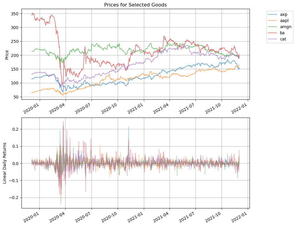
Plot Price and Returns Data#

prices.head()

	axp	aapl	amgn	ba	cat
Date
2019-12-04	113.070	64.105	214.000	346.777	130.179
2019-12-05	113.396	65.046	213.570	343.635	131.043
2019-12-06	115.629	66.302	213.900	351.996	132.594
2019-12-09	115.486	65.374	213.031	349.133	132.697
2019-12-10	115.907	65.756	213.964	345.842	132.734

fig, ax = plt.subplots(2, 1, figsize=(10, 10))
prices.plot(ax=ax[0], title='Prices for Selected Goods', xlabel="", ylabel="Price", grid=True, alpha=0.6)
ax[0].legend(loc='upper right', bbox_to_anchor=(1.2, 1.0))

returns = prices.diff()/prices.shift(1)
returns.plot(ax=ax[1], ylabel='Linear Daily Returns', xlabel="", grid=True, alpha=0.3, legend=False)

<AxesSubplot:ylabel='Linear Daily Returns'>

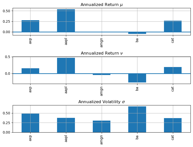
../../_images/05-portfolio-optimization_10_1.png

Linear and Log Returns#

returns = prices.diff()/prices.shift(1)

mu = (prices.diff()/prices.shift(1)).mean()
nu = np.log(prices).diff().mean()
sigma = np.log(prices).diff().std()

fig, ax = plt.subplots(3, 1, figsize=(8, 6))

(252*mu).plot(ax=ax[0], kind='bar', title='Annualized Return $\\mu$', grid=True)
ax[0].axhline(lw=2)

(252*nu).plot(ax=ax[1], kind='bar', title='Annualized Return $\\nu$', grid=True)
ax[1].axhline(lw=2)

(np.sqrt(252)*sigma).plot(ax=ax[2], kind='bar', title='Annualized Volatility $\\sigma$', grid=True)
fig.tight_layout()

../../_images/05-portfolio-optimization_12_0.png

print( "Annualized Returns and Standard Deviation\n")
print( "Symbol         mu           nu     mu-s^2/2        sigma")
for s in returns.columns.values.tolist():
    print(f"{s:5s}", end='')
    print(f"   {252.0*mu[s]:9.3f}", end='')
    print(f"    {252.0*nu[s]:9.3f}", end='')
    print(f"    {252.0*(mu[s] - 0.5*sigma[s]**2):9.3f}", end='')
    print(f"    {np.sqrt(252.0)*sigma[s]:9.3f}")

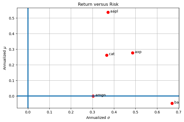
Annualized Returns and Standard Deviation

Symbol         mu           nu     mu-s^2/2        sigma
axp         0.276        0.157        0.158        0.486
aapl        0.536        0.467        0.467        0.372
amgn       -0.001       -0.047       -0.047        0.303
ba         -0.047       -0.270       -0.271        0.669
cat         0.262        0.195        0.195        0.366

Covariance and Correlation Matrices#

The covariance matrix is easily computed using the pandas .cov and .corr() functions.

cov = returns.cov()
rho = returns.corr()

pd.options.display.float_format = ' {:,.3f}'.format
print("\nAnnualized Covariance Matrix\n", 252*cov)
print("\nCorrelation Coefficients\n", rho)

Annualized Covariance Matrix
         axp   aapl   amgn     ba    cat
axp   0.244  0.080  0.057  0.234  0.123
aapl  0.080  0.138  0.061  0.103  0.054
amgn  0.057  0.061  0.093  0.050  0.050
ba    0.234  0.103  0.050  0.446  0.137
cat   0.123  0.054  0.050  0.137  0.133

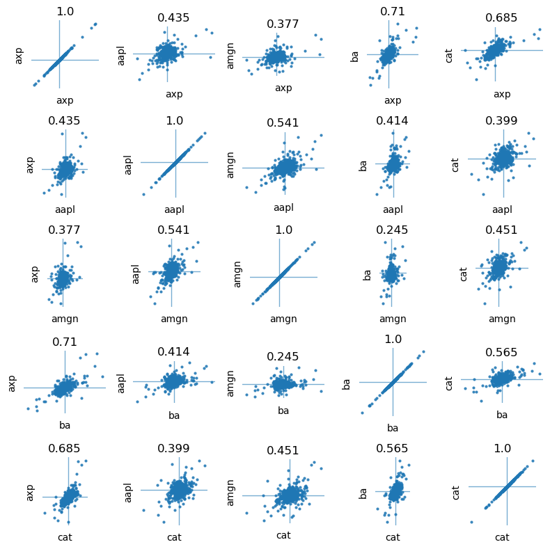
Correlation Coefficients
         axp   aapl   amgn     ba    cat
axp   1.000  0.435  0.377  0.710  0.685
aapl  0.435  1.000  0.541  0.414  0.399
amgn  0.377  0.541  1.000  0.245  0.451
ba    0.710  0.414  0.245  1.000  0.565
cat   0.685  0.399  0.451  0.565  1.000

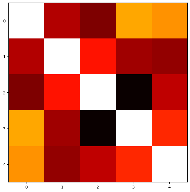
Visualizing the correlation coefficients#

syms = prices.columns
N = len(syms)

fig, ax = plt.subplots(N, N, figsize=(8, 8))
for i in range(0, N):
    for j in range(0, N):
        ax[i, j].plot(returns[syms[i]], returns[syms[j]], '.', ms=4, alpha=0.8)
        ax[i, j].axhline(0, lw=1, alpha=0.6)
        ax[i, j].axvline(0, lw=1, alpha=0.6)
        ax[i, j].axes.spines['top'].set_visible(False)
        ax[i, j].axes.spines['right'].set_visible(False)
        ax[i, j].axes.spines['bottom'].set_visible(False)
        ax[i, j].axes.spines['left'].set_visible(False)
        ax[i, j].axes.get_xaxis().set_ticks([])
        ax[i, j].axes.get_yaxis().set_ticks([])
        ax[i, j].set_xlabel(syms[i])
        ax[i, j].set_ylabel(syms[j])
        ax[i, j].set_aspect(1)
        ax[i, j].set_title(str(round(rho[syms[i]][syms[j]], 3)))
plt.tight_layout()

../../_images/05-portfolio-optimization_17_0.png

fig, ax = plt.subplots(1, 1, figsize=(8, 8))
ax.imshow(rho, cmap='hot', interpolation='nearest')

<matplotlib.image.AxesImage at 0x7fe96ab3b3d0>

../../_images/05-portfolio-optimization_18_1.png

Return versus Volatility#

plt.figure(figsize=(8, 5))
for s in returns.columns.values.tolist():
    plt.plot(np.sqrt(252.0)*sigma[s], 252*mu[s], 'r.', ms=15)
    plt.text(np.sqrt(252.0)*sigma[s], 252*mu[s], f"  {s:5<s}")

plt.axhline(0, lw=3)
plt.axvline(0, lw=3)
plt.xlim(-0.05, plt.xlim()[1])
plt.title('Return versus Risk')
plt.xlabel('Annualized $\sigma$')
plt.ylabel('Annualized $\mu$')
plt.grid(True)

../../_images/05-portfolio-optimization_20_0.png

Creating Portfolios#

A portfolio is created by allocating current wealth among a collection of assets. Let $w_n$ be the fraction of wealth allocated to the $n^{th}$ asset from a set of $N$ assets. Then

\[\sum_{n=1}^N w_n = 1\]

It may be possible to borrow assets, in which case the corresponding $w_n$ is negative. A long only portfolio is one such that all of weights $w_n$ are greater than or equal to zero.

Mean Return and Variance of a Portfolio#

Denoting the total value of the portfolio as V, the value invested in asset $n$ is $w_nV$. At a price $S_n$, the number of units of the asset is $\frac{w_nV}{S_n}$ for a total value

\[ V = \sum_{n=1}^N \frac{w_n V}{S_n}S_n \]

at the start of the investment period. The value of the investment at the end of the period, $V'$, is given by

\[ V' = \sum_{n=1}^N \frac{w_n V}{S_n}(1+r^{lin}_n)S_n \]

Taking differences we find

\[ V' - V = \sum_{n=1}^N \frac{w_n V}{S_n}r^{lin}_nS_n \]

which, after division, yields the return on the portfolio

\[ r^{lin}_p = \frac{V'-V}{V} = \sum_{n=1}^N w_nr^{lin}_n \]

Taking expectations, the mean return of the portfolio

\[\boxed{\bar{r}^{lin}_{p} = \sum_{n=1}^N w_n \bar{r}^{lin}_n}\]

Variance of portfolio return

\[\boxed{\sigma_{p}^2 = \sum_{m=1}^N\sum_{n=1}^N w_m w_n \sigma_{mn}}\]

Examples of Portfolios with Two Assets#

N_examples = 4

fig, ax = plt.subplots(N_examples, 1, figsize=(3, 10))

for i in range(0, N_examples):
    a, b = random.sample(prices.columns.values.tolist(), 2)

    for w in np.linspace(0.0, 1.0, 100):
        V = w*prices[a] + (1-w)*prices[b]
        rV = (V.diff()/V.shift(1)) 
        ax[i].plot(np.sqrt(252.0)*rV.std(), 252*rV.mean(),'g.', ms=5)
            
    for s in (a, b):    
        ax[i].plot(np.sqrt(252.0)*sigma[s], 252*mu[s], 'r.', ms=15)
        ax[i].text(np.sqrt(252.0)*sigma[s], 252*mu[s], "  {0:5<s}".format(s))

    ax[i].set_xlim(-0.05, 1.1*np.sqrt(252.0)*sigma.max())
    ax[i].set_ylim(1.1*252.0*mu.min(), 1.1*252.0*mu.max())

    ax[i].set_title('Return vs. Risk')
    ax[i].set_xlabel('$\sigma$')
    ax[i].set_ylabel('$r^{lin}$')
    ax[i].grid()

fig.tight_layout()

../../_images/05-portfolio-optimization_24_0.png

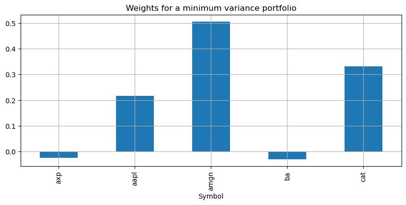
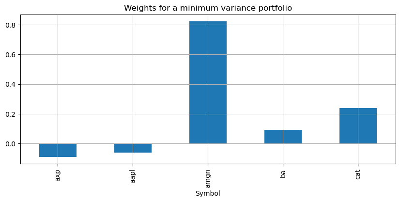
Minimum Risk Portfolio#

The minimum variance portfolio is found as a solution to $$\min_{w_1, w_2, \ldots, w_N} \sum_{m=1}^N\sum_{n=1}^N w_m w_n\sigma_{mn}$$ subject to $$\sum_{n=1}^N w_n = 1$$

Pyomo Model and Solution#

import pyomo.environ as pyo

# pyomo model
m = pyo.ConcreteModel()

# data
m.STOCKS = pyo.Set(initialize=returns.columns)

m.w = pyo.Var(m.STOCKS)

@m.Expression()
def portfolio_return(m):
    return sum(m.w[i] * mu[i] for i in m.STOCKS)

@m.Expression()
def portfolio_variance(m):
    return sum(m.w[i] * cov.loc[i, j] * m.w[j] for i in m.STOCKS for j in m.STOCKS)

@m.Objective(sense=pyo.minimize)
def minimum_variance(m):
    return m.portfolio_variance

@m.Constraint()
def weights(m):
    return sum(m.w[i] for i in m.STOCKS) == 1

# solve
pyo. SolverFactory('ipopt').solve(m)

# display solutions
w = pd.Series([m.w[i]() for i in m.STOCKS], m.STOCKS)

w.plot(kind='bar', figsize=(10, 4))
plt.xlabel('Symbol')
plt.title('Weights for a minimum variance portfolio')
plt.grid()

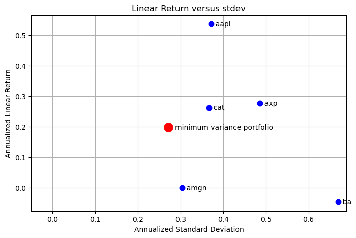
../../_images/05-portfolio-optimization_27_0.png

plt.figure(figsize=(8, 5))
for s in m.STOCKS:
    plt.plot(np.sqrt(252.0)*sigma[s], 252*mu[s], 'b.', ms=15)
    plt.text(np.sqrt(252.0)*sigma[s], 252*mu[s], "  {0:5<s}".format(s), va="center")

plt.plot(np.sqrt(252.0)*np.sqrt(m.portfolio_variance()), 252*m.portfolio_return(),
         'r.', ms=25)
plt.text(np.sqrt(252.0)*np.sqrt(m.portfolio_variance()), 252*m.portfolio_return(), 
         f"   minimum variance portfolio", va="center")
 
plt.xlim(-0.05, plt.xlim()[1])
plt.title('Linear Return versus stdev')
plt.xlabel('Annualized Standard Deviation')
plt.ylabel('Annualized Linear Return')
plt.grid(True)

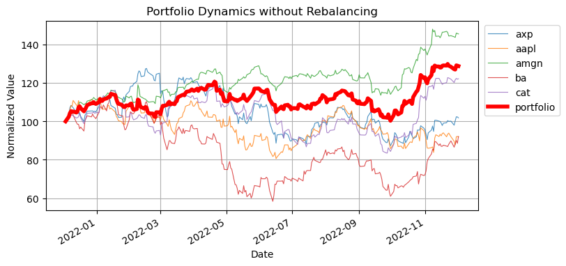
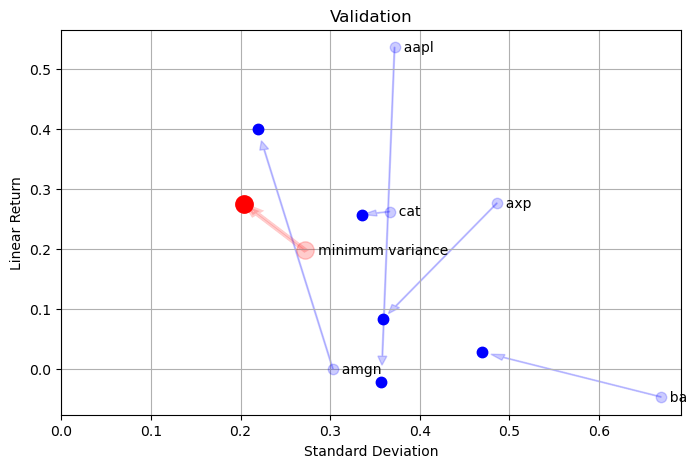
../../_images/05-portfolio-optimization_28_0.png

Out-of-Sample Testing#

Let’s test the performance of the minimum variance portfolio using out-of-sample price data.

# simulate portfolio of 100 units of currency
V = pd.Series(0, index=prices_test.index)
for s in m.STOCKS:
    V += (100.0*float(m.w[s]())/prices_test[s][0])*prices_test[s]
     
# plot reference stocks
for s in m.STOCKS:
    pd.Series(100.0*prices_test[s]/prices_test[s][0]).plot(lw=0.8, alpha=0.8)
     
V.plot(lw=4, figsize=(8, 4) ,color='red', label="portfolio", 
       title="Portfolio Dynamics without Rebalancing", ylabel="Normalized Value", grid=True)
plt.legend(loc='upper right', bbox_to_anchor=(1.2, 1.0))

<matplotlib.legend.Legend at 0x7fe96c462f40>

../../_images/05-portfolio-optimization_30_1.png

plt.figure(figsize=(8, 5))

returns_test = prices_test.diff()/prices_test.shift(1)
mu_test = returns_test.mean()
sigma_test = returns_test.std()

# plot stock components
for s in returns.columns:
    x = np.sqrt(252.0)*sigma[s]
    dx = np.sqrt(252.0)*(sigma_test[s] - sigma[s])
    y = 252.0*mu[s]
    dy = 252.0*(mu_test[s] - mu[s])
    
    plt.plot(x, y, 'b.', ms=15, alpha=0.2)
    plt.text(x, y, f"  {s:5<s}", va="center")
    
    plt.arrow(x, y, 0.95*dx, 0.95*dy, length_includes_head=True, head_width=0.01, color='b', alpha=0.2)
    plt.plot(x + dx, y + dy, 'b.', ms=15)

plt.xlim(0.0,plt.xlim()[1])
plt.title('Validation')
plt.xlabel('Standard Deviation')
plt.ylabel('Linear Return')
plt.grid(True)

x = np.sqrt(252.0)*np.sqrt(m.portfolio_variance())
y = 252*m.portfolio_return()
plt.plot(x, y, 'r.', ms=25, alpha=0.2)
plt.text(x, y, f"   minimum variance", va="center")

ReturnsV = (V.diff()/V.shift(1))
rlinMinVar = ReturnsV.mean()
stdevMinVar = ReturnsV.std()

dx = np.sqrt(252.0)*stdevMinVar - x
dy = 252.0*rlinMinVar - y

plt.plot(x + dx, y + dy, 'r.', ms=25)
plt.arrow(x, y, 0.95*dx, 0.95*dy, length_includes_head=True, head_width=0.01, color='r', lw=3, alpha=0.2)

<matplotlib.patches.FancyArrow at 0x7fe96c929b20>

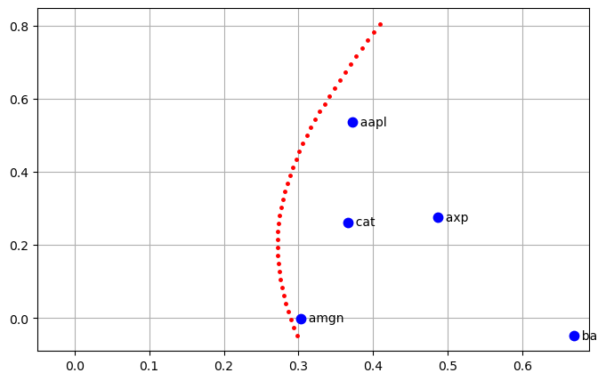
../../_images/05-portfolio-optimization_31_1.png

Markowitz Portfolio#

The minimum variance portfolio does a good job of handling volatility, but at the expense of relatively low return. The Markowitz portfolio adds an additional constraint to specify mean portfolio return. $$\min_{w_1, w_2, \ldots, w_N} \sum_{m=1}^N\sum_{n=1}^N w_m w_n\sigma_{mn}$$ subject to $$\sum_{n=1}^N w_n = 1$$ and $$\sum_{n=1}^N w_n \bar{r}^{lin}_n = \bar{r}^{lin}_p$$ By programming the solution of the optimization problem as a function of $\bar{r}_p$, it is possible to create a risk-return tradeoff curve.

import pyomo.environ as pyo

def markowitz_model(returns, cov, rp=None):
    
    m = pyo.ConcreteModel()
    
    m.rp = pyo.Param(initialize=rp, mutable=True)

    m.STOCKS = pyo.Set(initialize=returns.columns)
    m.w = pyo.Var(m.STOCKS)

    @m.Expression()
    def portfolio_return(m):
        return sum(m.w[i] * mu[i] for i in m.STOCKS)

    @m.Expression()
    def portfolio_variance(m):
        return sum(m.w[i] * cov.loc[i, j] * m.w[j] for i in m.STOCKS for j in m.STOCKS)

    @m.Objective(sense=pyo.minimize)
    def minimum_variance(m):
        return m.portfolio_variance

    @m.Constraint()
    def weights(m):
        return sum(m.w[i] for i in m.STOCKS) == 1
    
    @m.Constraint()
    def ma(m):
        if m.rp is not None:
            return m.portfolio_return == m.rp
        else:
            return pyo.Constraint.Skip

    # solve
    pyo. SolverFactory('ipopt').solve(m)

    return(m)

m = markowitz_model(returns, cov, 0.0/252)
w = pd.Series([m.w[i]() for i in m.STOCKS], m.STOCKS)
w.plot(kind='bar', figsize=(10, 4))
plt.xlabel('Symbol')
plt.title('Weights for a minimum variance portfolio')
plt.grid()

../../_images/05-portfolio-optimization_33_0.png

fig, ax = plt.subplots(1, 1, figsize=(8, 5))
for s in m.STOCKS:
    ax.plot(np.sqrt(252.0)*sigma[s], 252*mu[s], 'b.', ms=15)
    ax.text(np.sqrt(252.0)*sigma[s], 252*mu[s], "  {0:5<s}".format(s), va="center")

m = markowitz_model(returns, cov, 0/252)
solver = pyo.SolverFactory('ipopt')

# scan solution as function of portfolio return
for rp in np.linspace(min(0, mu.min()), 1.5*mu.max(), 40):
    m.rp.value = rp
    solver.solve(m)
    x = np.sqrt(252 * m.portfolio_variance())
    y = 252 * m.portfolio_return()
    ax.plot(x, y, 'r.', ms=5)
    
ax.set_xlim(-0.05, )
ax.grid(True)

../../_images/05-portfolio-optimization_34_0.png

Markowitz Portfolio without Shorting#

At this point there are no constraints on portfolio weights $w_1, w_2, \ldots, w_N$ other than they must sum to one. It is possible for the solution to the minimum variance or Markowitz portfolio problems to include negative weights, or weights greater than one. A negative weight corresponds to short selling an asset within the portfolio. A weight greater than one implies that short selling has taken place and the proceeds used to buy a stake in another asset that is greater in value than the portfolio. These are aggressive investment strategies.

A common constraint on operators or investors will accept short selling as a business strategy.

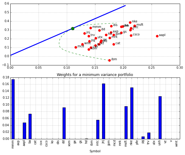
Risk-Free Asset#

The minimum variance portfolio does a good job of handling volatility, but at the expense of relatively low return. The Markowitz portfolio adds an additional constraint to specify mean portfolio return. $$\min_{w_1, w_2, \ldots, w_N} \sum_{m=1}^N\sum_{n=1}^N w_m w_n\sigma_{mn}$$ subject to $$\sum_{n=1}^N w_n = 1 - w_f$$ and $$\sum_{n=1}^N w_n \bar{r}^{lin}_n + w_f r_f = \bar{r}^{lin}_p$$ By programming the solution of the optimization problem as a function of $\bar{r}_p$, it is possible to create a risk-return tradeoff curve.

# cvxpy problem description

m = ConcreteModel()

m.w = Var(range(0,N), domain = Reals)
wf

w = cvx.Variable(N)
wf = cvx.Variable(1)
r = cvx.Parameter()

rf = 0.01/252.0

risk = cvx.quad_form(w, np.array(sigma))
prob = cvx.Problem(cvx.Minimize(risk), 
               [cvx.sum_entries(w) == 1 - wf, 
                np.array(rlin).T*w + wf*rf == r,
               w >= 0])

# lists to store results of parameter scans
r_data_rf = []
stdev_data_rf = []
w_data_rf = []

# scan solution as function of portfolio return
for rp in np.linspace(np.min(rf,rlin.min()),1.5*rlin.max(),100):
    r.value = rp
    s = prob.solve()
    if prob.status == "optimal":
        r_data_rf.append(rp)
        stdev_data_rf.append(np.sqrt(prob.solve()))
        w_data_rf.append([u[0,0] for u in w.value])

plt.figure(figsize=(10,8))
plt.subplot(211)
plt.plot(np.sqrt(252.0)*np.array(stdev_data_rf), 252.0*np.array(r_data_rf),lw=3)
plt.plot(np.sqrt(252.0)*np.array(stdev_data), 252.0*np.array(r_data),'g--')
for s in syms:
    plt.plot(np.sqrt(252.0)*stdev[s],252.0*rlin[s],'r.',ms=15)
    plt.text(np.sqrt(252.0)*stdev[s],252.0*rlin[s],"  {0:5<s}".format(s))
    
# find max Sharpe ratio
k = np.argmax(np.divide(np.array(r_data)-rf,np.array(stdev_data)))
smax = stdev_data[k]
rmax = r_data[k]
plt.plot(np.sqrt(252.0)*smax,252.0*rmax,'o',ms=10)
print 252.0*rmax
print 252.0*rf
print np.sqrt(252.0)*smax

plt.xlim(0.0,plt.xlim()[1])
plt.grid()

plt.subplot(212)

wval = pd.Series(w_data[k],syms)
wval.plot(kind='bar')

plt.xlabel('Symbol')
plt.title('Weights for a minimum variance portfolio')
plt.grid()

319026600441
01
110681042214

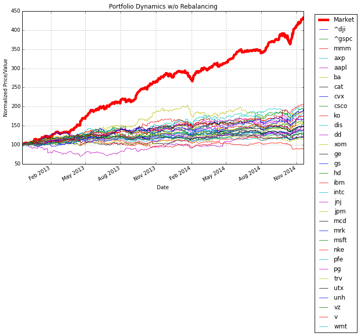
../../_images/05-portfolio-optimization_38_1.png

N = len(Prices.columns.values.tolist())

# create price history of the portfolio
V = pd.Series(0,index=Prices.index,name='Market')
for s in Prices.columns.values.tolist():
    V += (100.0*float(wval[s])/Prices[s][0])*Prices[s]
    
V.plot(lw=5,figsize=(10,6),color='red')

# plot components
plt.hold(True)
for s in Prices.columns.values.tolist():
    S = pd.Series(100.0*Prices[s]/Prices[s][0])
    S.plot(lw=0.8)

plt.legend(loc='upper right',bbox_to_anchor=(1.2, 1.0))
plt.title('Portfolio Dynamics w/o Rebalancing')
plt.ylabel('Normalized Price/Value')
plt.grid()

../../_images/05-portfolio-optimization_40_0.png

P['Market'] = V
Sigma = P.cov()
Sigma.ix[:,'Market']/Sigma.ix['Market','Market']

^dji     12.528858
^gspc     1.934181
mmm       0.197222
axp       0.120742
aapl      0.133096
ba        0.208771
cat       0.072742
cvx       0.051164
csco      0.016654
ko        0.016795
dis       0.136692
dd        0.086136
xom       0.053090
ge        0.020513
gs        0.154648
hd        0.086056
ibm      -0.047416
intc      0.046451
jnj       0.122271
jpm       0.054673
mcd       0.023521
mrk       0.067638
msft      0.068685
nke       0.121157
pfe       0.016580
pg        0.048426
trv       0.075682
utx       0.104676
unh       0.123136
vz        0.022144
v         0.065840
wmt       0.029284
Market    1.000000
Name: Market, dtype: float64

Maximum Log Return (to be developed).#

import cvxpy as cvx

N = len(syms)

w = cvx.Variable(N)
risk = cvx.quad_form(w, np.array(sigma))
prob = cvx.Problem(cvx.Maximize(np.array(rlin).T*w-0.5*risk), 
               [cvx.sum_entries(w) == 1,
                risk <= 0.0005/np.sqrt(252.0),
                w>=0])

prob.solve()
print prob.status

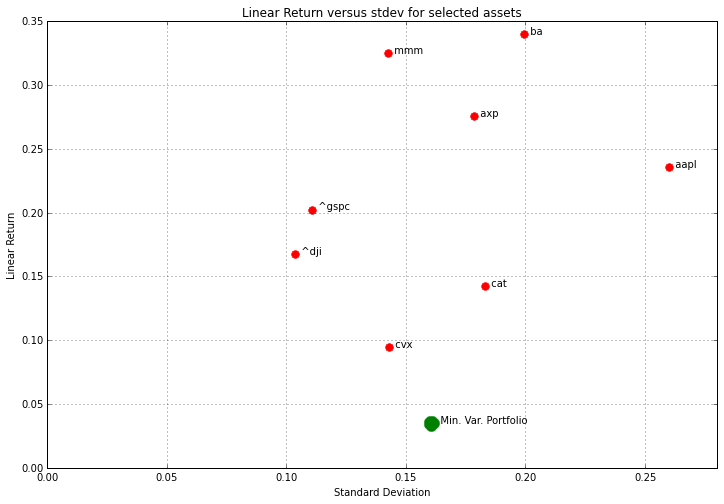
plt.figure(figsize=(12,8))
for s in Returns.columns.values.tolist():
    plt.plot(np.sqrt(252.0)*stdev[s],252*rlin[s],'r.',ms=15)
    plt.text(np.sqrt(252.0)*stdev[s],252*rlin[s],"  {0:5<s}".format(s))

plt.xlim(0.0,plt.xlim()[1])
plt.title('Linear Return versus stdev for selected assets')
plt.xlabel('Standard Deviation')
plt.ylabel('Linear Return')
plt.grid()
plt.hold(True)

plt.plot(np.sqrt(252.0)*stdevMinVar,252.0*rlinMinVar,'g.',ms=30)
plt.text(np.sqrt(252.0)*stdevMinVar,252.0*rlinMinVar,'   Min. Var. Portfolio')

wval = np.array(w.value)[:,0].T
rlog = np.dot(np.array(rlin).T,wval)
stdevlog = np.sqrt(np.dot(np.dot(wval,np.array(sigma)),wval))

plt.plot(np.sqrt(252.0)*stdevlog,252.0*rlog,'g.',ms=30)
plt.text(np.sqrt(252.0)*stdevlog,252.0*rlog,'  Max. Return Portfolio')

infeasible

---------------------------------------------------------------------------
IndexError                                Traceback (most recent call last)
<ipython-input-353-221d4f60194f> in <module>()
     28 plt.text(np.sqrt(252.0)*stdevMinVar,252.0*rlinMinVar,'   Min. Var. Portfolio')
     29 
---> 30 wval = np.array(w.value)[:,0].T
     31 rlog = np.dot(np.array(rlin).T,wval)
     32 stdevlog = np.sqrt(np.dot(np.dot(wval,np.array(sigma)),wval))

IndexError: too many indices for array

../../_images/05-portfolio-optimization_43_2.png

Exercises#

Modify the minimum variance portfolio to be ‘long-only’, and add a diversification constraints that no more than 20% of the portfolio can be invested in any single asset. How much does this change the annualized return? the annualized standard deviation?
Modify the Markowitz portfolio to allow long-only positions and a diversification constraint that no more than 20% of the portfolio can be invested in any single asset. What conclusion to you draw?

CBE 40455/60455 Process Operations

Portfolio Optimization

Contents