
2.5. Gasoline Blending#
Keywords: blending, cbc usage
The task is to determine the most profitable blend of gasoline products from given set of refinery streams.
Source: Olsen, T. (2014, May). An Oil Refinery Walk-Through. Chemical Engineering Progress, 34-40. pdf available here.
2.5.1. Imports#
import pandas as pd

import shutil
import sys
import os.path

if not shutil.which("pyomo"):
    !pip install -q pyomo
    assert(shutil.which("pyomo"))

if not (shutil.which("cbc") or os.path.isfile("cbc")):
    if "google.colab" in sys.modules:
        !apt-get install -y -qq coinor-cbc
    else:
        try:
            !conda install -c conda-forge coincbc
        except:
            pass

assert(shutil.which("cbc") or os.path.isfile("cbc"))

import pyomo.environ as pyomo
2.5.2. Gasoline product specifications#
The gasoline products include regular and premium gasoline. In addition to the current price, the specifications include
octane the minimum road octane number. Road octane is the computed as the average of the Research Octane Number (RON) and Motor Octane Number (MON).
Reid Vapor Pressure Upper and lower limits are specified for the Reid vapor pressure. The Reid vapor pressure is the absolute pressure exerted by the liquid at 100°F.
benzene the maximum volume percentage of benzene allowed in the final product. Benzene helps to increase octane rating, but is also a treacherous environmental contaminant.
products = {
    'Regular' : {'price': 2.75, 'octane': 87, 'RVPmin': 0.0, 'RVPmax': 15.0, 'benzene': 1.1},
    'Premium' : {'price': 2.85, 'octane': 91, 'RVPmin': 0.0, 'RVPmax': 15.0, 'benzene': 1.1},
}

print(pd.DataFrame.from_dict(products).T)
         RVPmax  RVPmin  benzene  octane  price
Regular    15.0     0.0      1.1    87.0   2.75
Premium    15.0     0.0      1.1    91.0   2.85
2.5.3. Stream specifications#
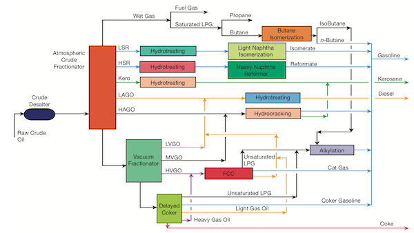
A typical refinery produces many intermediate streams that can be incorporated in a blended gasoline product. Here we provide data on seven streams that include:
Butane n-butane is a C4 product stream produced from the light components of the crude being processed by the refinery. Butane is a highly volatile of gasoline.
LSR Light straight run naptha is a 90°F to 190°F cut from the crude distillation column primarily consisting of straight chain C5-C6 hydrocarbons.
Isomerate is the result of isomerizing LSR to produce branched molecules that results in higher octane number.
Reformate is result of catalytic reforming heavy straight run napthenes to produce a high octane blending component, as well by-product hydrogen used elsewhere in the refinery for hydro-treating.
Reformate LB is a is a low benzene variant of reformate.
FCC Naphta is the product of a fluidized catalytic cracking unit designed to produce gasoline blending components from long chain hydrocarbons present in the crude oil being processed by the refinery.
Alkylate The alkylation unit reacts iso-butane with low-molecular weight alkenes to produce a high octane blending component for gasoline.
The stream specifications include research octane and motor octane numbers for each blending component, the Reid vapor pressure, the benzene content, cost, and availability (in gallons per day). The road octane number is computed as the average of the RON and MON.
streams = {
    'Butane'       : {'RON': 93.0, 'MON': 92.0, 'RVP': 54.0, 'benzene': 0.00, 'cost': 0.85, 'avail': 30000},
    'LSR'          : {'RON': 78.0, 'MON': 76.0, 'RVP': 11.2, 'benzene': 0.73, 'cost': 2.05, 'avail': 35000},
    'Isomerate'    : {'RON': 83.0, 'MON': 81.1, 'RVP': 13.5, 'benzene': 0.00, 'cost': 2.20, 'avail': 0},
    'Reformate'    : {'RON':100.0, 'MON': 88.2, 'RVP':  3.2, 'benzene': 1.85, 'cost': 2.80, 'avail': 60000},
    'Reformate LB' : {'RON': 93.7, 'MON': 84.0, 'RVP':  2.8, 'benzene': 0.12, 'cost': 2.75, 'avail': 0},
    'FCC Naphtha'  : {'RON': 92.1, 'MON': 77.1, 'RVP':  1.4, 'benzene': 1.06, 'cost': 2.60, 'avail': 70000},
    'Alkylate'     : {'RON': 97.3, 'MON': 95.9, 'RVP':  4.6, 'benzene': 0.00, 'cost': 2.75, 'avail': 40000},
}

# calculate road octane as (R+M)/2
for s in streams.keys():
    streams[s]['octane'] = (streams[s]['RON'] + streams[s]['MON'])/2

# display feed information
print(pd.DataFrame.from_dict(streams).T)
               MON    RON   RVP    avail  benzene  cost  octane
Butane        92.0   93.0  54.0  30000.0     0.00  0.85   92.50
LSR           76.0   78.0  11.2  35000.0     0.73  2.05   77.00
Isomerate     81.1   83.0  13.5      0.0     0.00  2.20   82.05
Reformate     88.2  100.0   3.2  60000.0     1.85  2.80   94.10
Reformate LB  84.0   93.7   2.8      0.0     0.12  2.75   88.85
FCC Naphtha   77.1   92.1   1.4  70000.0     1.06  2.60   84.60
Alkylate      95.9   97.3   4.6  40000.0     0.00  2.75   96.60
2.5.4. Blending model#
This simplified blending model assumes the product attributes can be computed as linear volume weighted averages of the component properties. Let the decision variable \(x_{s,p} \geq 0\) be the volume, in gallons, of blending component \(s \in S\) used in the final product \(p \in P\).
The objective is maximize profit, which is the difference between product revenue and stream costs.
or $\( \begin{align} \mbox{profit} & = \max_{x_{s,p}}\left( \sum_{p\in P} \sum_{s\in S} x_{s,p}\mbox{Price}_p - \sum_{p\in P} \sum_{s\in S} x_{s,p}\mbox{Cost}_s \right) \end{align} \)$
The blending constraint for octane can be written as
where \(\mbox{Octane}_s\) refers to the octane rating of stream \(s\), whereas \(\mbox{Octane}_p\) refers to the octane rating of product \(p\). Multiplying through by the denominator, and consolidating terms gives
The same assumptions and development apply to the benzene constraint
Reid vapor pressure, however, follows a somewhat different mixing rule. For the Reid vapor pressure we have
2.5.5. Pyomo implementation#
This model is implemented in the following cell.
# create model
m = pyomo.ConcreteModel()

# create decision variables
S = streams.keys()
P = products.keys()
m.x = pyomo.Var(S,P, domain=pyomo.NonNegativeReals)

# objective
revenue = sum(sum(m.x[s,p]*products[p]['price'] for s in S) for p in P)
cost = sum(sum(m.x[s,p]*streams[s]['cost'] for s in S) for p in P)
m.profit = pyomo.Objective(expr = revenue - cost, sense=pyomo.maximize)

# constraints
m.cons = pyomo.ConstraintList()
for s in S:
    m.cons.add(sum(m.x[s,p] for p in P) <= streams[s]['avail'])
for p in P:
    m.cons.add(sum(m.x[s,p]*(streams[s]['octane'] -    products[p]['octane'])       for s in S) >= 0)
    m.cons.add(sum(m.x[s,p]*(streams[s]['RVP']**1.25 - products[p]['RVPmin']**1.25) for s in S) >= 0)
    m.cons.add(sum(m.x[s,p]*(streams[s]['RVP']**1.25 - products[p]['RVPmax']**1.25) for s in S) <= 0)
    m.cons.add(sum(m.x[s,p]*(streams[s]['benzene'] -   products[p]['benzene'])      for s in S) <= 0)

# solve
solver = pyomo.SolverFactory('cbc')
solver.solve(m)

# display results
vol = sum(m.x[s,p]() for s in S for p in P)
print("Total Volume =", round(vol, 1), "gallons.")
print("Total Profit =", round(m.profit(), 1), "dollars.")
print("Profit =", round(100*m.profit()/vol,1), "cents per gallon.")
Total Volume = 235000.0 gallons.
Total Profit = 100425.0 dollars.
Profit = 42.7 cents per gallon.
2.5.6. Displaying the solution#
2.5.6.1. by refinery stream#
stream_results = pd.DataFrame()
for s in S:
    for p in P:
        stream_results.loc[s,p] = round(m.x[s,p](), 1)
    stream_results.loc[s,'Total'] = round(sum(m.x[s,p]() for p in P), 1)
    stream_results.loc[s,'Available'] = streams[s]['avail']

stream_results['Unused (Slack)'] = stream_results['Available'] - stream_results['Total']
print(stream_results)
              Regular  Premium    Total  Available  Unused (Slack)
Butane        21754.6   8245.4  30000.0    30000.0             0.0
LSR            9211.6  25788.4  35000.0    35000.0             0.0
Isomerate         0.0      0.0      0.0        0.0             0.0
Reformate     19783.9  40216.1  60000.0    60000.0             0.0
Reformate LB      0.0      0.0      0.0        0.0             0.0
FCC Naphtha   70000.0      0.0  70000.0    70000.0             0.0
Alkylate         -0.0  40000.0  40000.0    40000.0             0.0
2.5.6.2. by refinery product#
product_results = pd.DataFrame()
for p in P:
    product_results.loc[p,'Volume'] = round(sum(m.x[s,p]() for s in S), 1)
    product_results.loc[p,'octane'] = round(sum(m.x[s,p]()*streams[s]['octane'] for s in S)
                                            /product_results.loc[p,'Volume'], 1)
    product_results.loc[p,'RVP'] = round((sum(m.x[s,p]()*streams[s]['RVP']**1.25 for s in S)
                                            /product_results.loc[p,'Volume'])**0.8, 1)
    product_results.loc[p,'benzene'] = round(sum(m.x[s,p]()*streams[s]['benzene'] for s in S)
                                            /product_results.loc[p,'Volume'], 1)
print(product_results)
           Volume  octane   RVP  benzene
Regular  120750.0    87.0  15.0      1.0
Premium  114250.0    91.0  10.6      0.8
2.5.7. Exercises#
2.5.7.1. 1. Expand product list with mid-grade gasoline#
The marketing team says there is an opportunity to create a mid-grade gasoline product with a road octane number of 89 that would sell for $2.82/gallon, and with all other specifications the same. Could an additional profit be created?
Create a new cell (or cells) below to compute a solution to this exercise.
2.5.7.2. 2. Impact of regulatory change#
New environmental regulations have reduced the allowable benzene levels from 1.1 vol% to 0.62 vol%, and the maximum Reid vapor pressure from 15.0 to 9.0.
Compared to the base case (i.e., without the midgrade product), how does this change profitability?
2.5.7.3. 3. Impact of a change in refinery operations#
Given the new product specifications in Exercise 2, let’s consider using different refinery streams. In place of Reformate, the refinery could produce Reformate LB. (That is, one or the other of the two streams could be 60000 gallons per day, but not both). Same for LSR and Isomerate. How should the refinery be operated to maximize profitability? (Hint: You will need to introduce at least two extra decision variables corresponding to the decisions to use the alternative processes.)
2.5.7.4. Mini-Project: Transfer Pricing (Sensitivity Analysis)#
The profitability of this refinery is determined by the amount of each blending stream that is available. It may be possible to purchase additional quantities of each stream in the market. Assume the pre-conditions of exercises 1, 2, and 3 are all in effect. Also assume that all seven streams could be available for purchase and blending even if they are not produced in the refinery.
What is the maximum price you would be willing to pay for each of the seven streams?