5.1. Response of a First Order System to Step and Square Wave Inputs#
Keywords: Simulator, ipopt usage
This notebook demonstrates simulation of a linear first-order system in Pyomo using the Simulator class from Pyomo. The notebook also demonstrates the construction and use of analytical approximations to step functions and square wave inputs.
5.1.1. Imports#
import matplotlib.pyplot as plt

from math import pi

import shutil
import sys
import os.path

if not shutil.which("pyomo"):
    !pip install -q pyomo
    assert(shutil.which("pyomo"))

if not (shutil.which("ipopt") or os.path.isfile("ipopt")):
    if "google.colab" in sys.modules:
        !wget -N -q "https://ampl.com/dl/open/ipopt/ipopt-linux64.zip"
        !unzip -o -q ipopt-linux64
    else:
        try:
            !conda install -c conda-forge ipopt
        except:
            pass

assert(shutil.which("ipopt") or os.path.isfile("ipopt"))

from pyomo.environ import *
from pyomo.dae import *
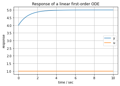
5.1.2. First-order differential equation with constant input#
The following cell simulates the response of a first-order linear model in the form
where \(\tau\) and \(K\) are model parameters, and \(u(t)=1\) is an external process input.
tfinal = 10
tau = 1
K = 5

# define u(t)
def u(t):
    return 1.0

# create a model object
model = ConcreteModel()

# define the independent variable
model.t = ContinuousSet(bounds=(0, tfinal))

# define the dependent variables
model.y = Var(model.t)
model.dydt = DerivativeVar(model.y)

# fix the initial value of y
model.y[0].fix(4)

# define the differential equation as a constraint
@model.Constraint(model.t)
def ode(m, t):
    return tau*model.dydt[t] + model.y[t] == K*u(t)
model.y.display()
y : Size=2, Index=t
    Key : Lower : Value : Upper : Fixed : Stale : Domain
      0 :  None :     4 :  None :  True : False :  Reals
     10 :  None :  None :  None : False :  True :  Reals
# simulation using scipy integrators
tsim, profiles = Simulator(model, package='scipy').simulate(numpoints=101)
tsim
profiles
array([[4.        ],
       [4.09516518],
       [4.18126635],
       [4.25917761],
       [4.32967597],
       [4.39346666],
       [4.45118776],
       [4.50341441],
       [4.55067095],
       [4.5934305 ],
       [4.63212104],
       [4.66713048],
       [4.69880924],
       [4.72747142],
       [4.75340218],
       [4.77686354],
       [4.79809743],
       [4.81731337],
       [4.83469911],
       [4.85042886],
       [4.86466192],
       [4.87754068],
       [4.88919421],
       [4.89973902],
       [4.90928022],
       [4.91791317],
       [4.92572462],
       [4.93279283],
       [4.93918842],
       [4.9449753 ],
       [4.95021132],
       [4.95494926],
       [4.95923631],
       [4.96311531],
       [4.9666254 ],
       [4.96980139],
       [4.97267511],
       [4.97527546],
       [4.97762825],
       [4.97975715],
       [4.98168354],
       [4.98342653],
       [4.9850037 ],
       [4.9864308 ],
       [4.98772205],
       [4.98889045],
       [4.98994758],
       [4.99090399],
       [4.99176946],
       [4.99255276],
       [4.99326147],
       [4.99390272],
       [4.99448304],
       [4.99500813],
       [4.99548319],
       [4.99591304],
       [4.99630201],
       [4.99665391],
       [4.99697229],
       [4.99726045],
       [4.99752118],
       [4.99775709],
       [4.99797055],
       [4.99816375],
       [4.99833848],
       [4.99849659],
       [4.99863967],
       [4.9987691 ],
       [4.99888618],
       [4.99899214],
       [4.99908806],
       [4.99917492],
       [4.99925359],
       [4.99932482],
       [4.99938923],
       [4.99944739],
       [4.99950001],
       [4.99954764],
       [4.99959071],
       [4.99962961],
       [4.99966475],
       [4.99969657],
       [4.99972537],
       [4.99975145],
       [4.99977533],
       [4.99979649],
       [4.99981579],
       [4.99983331],
       [4.99984916],
       [4.99986348],
       [4.99987643],
       [4.99988812],
       [4.99989869],
       [4.99990825],
       [4.99991692],
       [4.99992473],
       [4.99993178],
       [4.99993818],
       [4.999944  ],
       [4.99994935],
       [4.99995422]])
fig, ax = plt.subplots(1, 1)
ax.plot(tsim, profiles, label='y')
ax.plot(tsim, [u(t) for t in tsim], label='u')
ax.set_xlabel('time / sec')
ax.set_ylabel('response')
ax.set_title('Response of a linear first-order ODE')
ax.legend()
ax.grid(True)
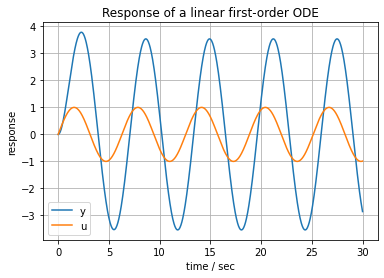
5.1.3. Encapsulating into a function#
In following cells we would like to explore the response of a first order system to changes in parameters and input functions. To facilitate this study, the next cell encapsulates the simulation into a function that can be called with different parameter values and input functions.
def first_order(K=1, tau=1, tfinal=1, u=lambda t: 1):
    model = ConcreteModel()
    model.t = ContinuousSet(bounds=(0, tfinal))
    model.y = Var(model.t)
    model.dydt = DerivativeVar(model.y)
    model.y[0].fix(0)
    @model.Constraint(model.t)
    def ode(m, t):
        return tau*model.dydt[t] + model.y[t] == K*u(t)

    tsim, profiles = Simulator(model, package='scipy').simulate(numpoints=1000)

    fig, ax = plt.subplots(1, 1)
    ax.plot(tsim, profiles, label='y')
    ax.plot(tsim, [u(t) for t in tsim], label='u')
    ax.set_xlabel('time / sec')
    ax.set_ylabel('response')
    ax.set_title('Response of a linear first-order ODE')
    ax.legend()
    ax.grid(True)

first_order(5, 1, 30, sin)
5.1.4. Analytical approximation to a step input#
The math functions supported by Pyomo are limited to that are imported to the standard arithmetic operations of Python (*, /, *, *=, /=, *=) and a particular set of nonlinear functions from the Python math library. Simulating the response of a system to a discontinuous step input, for example, requires an approximate.
An infinitely differentiable approximation to a step change is given by the Butterworth function \(b_n(t)\)
where \(n\) is the order of a approximation, and \(c\) is value of \(t\) where the step change occurs.
u = lambda t: 1/(1 + (t/10)**100)

first_order(5, 1, 30, u)
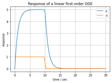
u = lambda t: 1 - 1/(1 + (t/10)**100)

first_order(5, 1, 30, u)

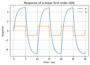
5.1.5. Analytical approximation to a square wave input#
An analytical approximation to a square wave with frequency \(f\) is given by
where the first term is the Lanczos sigma factor designed to suppress the Gibb’s phenomenon associated with Fourier series approximations.
def square(t, f=1, N=31):
    return (4/pi)*sum((N*sin(k*pi/N)/k/pi)*sin(2*k*f*pi*t)/k for k in range(1, N+1,2))

u = lambda t: square(t, 0.1)

first_order(5, 1, 30, u)