5.3. Transient Heat Conduction in Various Geometries#
Keywords: ipopt usage, dae, differential-algebraic equations, pde, partial differential equations
5.3.1. Imports#
%matplotlib inline

import numpy as np
import matplotlib.pyplot as plt
from mpl_toolkits.mplot3d.axes3d import Axes3D

import shutil
import sys
import os.path

if not shutil.which("pyomo"):
    !pip install -q pyomo
    assert(shutil.which("pyomo"))

if not (shutil.which("ipopt") or os.path.isfile("ipopt")):
    if "google.colab" in sys.modules:
        !wget -N -q "https://ampl.com/dl/open/ipopt/ipopt-linux64.zip"
        !unzip -o -q ipopt-linux64
    else:
        try:
            !conda install -c conda-forge ipopt
        except:
            pass

assert(shutil.which("ipopt") or os.path.isfile("ipopt"))
from pyomo.environ import *
from pyomo.dae import *
5.3.2. Rescaling the heat equation#
Transport of heat in a solid is described by the familiar thermal diffusion model
We’ll assume the thermal conductivity \(k\) is a constant, and define thermal diffusivity in the conventional way
We will further assume symmetry with respect to all spatial coordinates except \(r\) where \(r\) extends from \(-R\) to \(+R\). The boundary conditions are
where we have assumed symmetry with respect to \(r\) and uniform initial conditions \(T(0, r) = T_0\) for all \(0 \leq r \leq R\). Following standard scaling procedures, we introduce the dimensionless variables
5.3.3. Dimensionless model#
Under these conditions the problem reduces to
with auxiliary conditions
which we can specialize to specific geometries.
5.3.4. Preliminary code#
def model_plot(m):
    r = sorted(m.r)
    t = sorted(m.t)

    rgrid = np.zeros((len(t), len(r)))
    tgrid = np.zeros((len(t), len(r)))
    Tgrid = np.zeros((len(t), len(r)))

    for i in range(0, len(t)):
        for j in range(0, len(r)):
            rgrid[i,j] = r[j]
            tgrid[i,j] = t[i]
            Tgrid[i,j] = m.T[t[i], r[j]].value

    fig = plt.figure(figsize=(10,6))
    ax = fig.add_subplot(1, 1, 1, projection='3d')
    ax.set_xlabel('Distance r')
    ax.set_ylabel('Time t')
    ax.set_zlabel('Temperature T')
    p = ax.plot_wireframe(rgrid, tgrid, Tgrid)
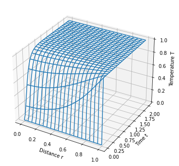
5.3.5. Planar coordinates#
Suppressing the prime notation, for a slab geometry the model specializes to
with auxiliary conditions
m = ConcreteModel()

m.r = ContinuousSet(bounds=(0,1))
m.t = ContinuousSet(bounds=(0,2))

m.T = Var(m.t, m.r)

m.dTdt   = DerivativeVar(m.T, wrt=m.t)
m.dTdr   = DerivativeVar(m.T, wrt=m.r)
m.d2Tdr2 = DerivativeVar(m.T, wrt=(m.r, m.r))

@m.Constraint(m.t, m.r)
def pde(m, t, r):
    if t == 0:
        return Constraint.Skip
    if r == 0 or r == 1:
        return Constraint.Skip
    return m.dTdt[t,r] == m.d2Tdr2[t,r]

m.obj = Objective(expr=1)

m.ic  = Constraint(m.r, rule=lambda m, r:    m.T[0,r] == 0 if r > 0 and r < 1 else Constraint.Skip)
m.bc1 = Constraint(m.t, rule=lambda m, t:    m.T[t,1] == 1)
m.bc2 = Constraint(m.t, rule=lambda m, t: m.dTdr[t,0] == 0)

TransformationFactory('dae.finite_difference').apply_to(m, nfe=50, scheme='FORWARD', wrt=m.r)
TransformationFactory('dae.finite_difference').apply_to(m, nfe=50, scheme='FORWARD', wrt=m.t)
SolverFactory('ipopt').solve(m, tee=True).write()
model_plot(m)
Ipopt 3.13.4:

******************************************************************************
This program contains Ipopt, a library for large-scale nonlinear optimization.
 Ipopt is released as open source code under the Eclipse Public License (EPL).
         For more information visit https://github.com/coin-or/Ipopt
******************************************************************************

This is Ipopt version 3.13.4, running with linear solver mumps.
NOTE: Other linear solvers might be more efficient (see Ipopt documentation).

Number of nonzeros in equality constraint Jacobian...:    30347
Number of nonzeros in inequality constraint Jacobian.:        0
Number of nonzeros in Lagrangian Hessian.............:        0

Total number of variables............................:    10299
                     variables with only lower bounds:        0
                variables with lower and upper bounds:        0
                     variables with only upper bounds:        0
Total number of equality constraints.................:    10200
Total number of inequality constraints...............:        0
        inequality constraints with only lower bounds:        0
   inequality constraints with lower and upper bounds:        0
        inequality constraints with only upper bounds:        0

iter    objective    inf_pr   inf_du lg(mu)  ||d||  lg(rg) alpha_du alpha_pr  ls
   0  1.0000000e+00 1.00e+00 0.00e+00  -1.0 0.00e+00    -  0.00e+00 0.00e+00   0
   1  1.0000000e+00 1.48e-12 2.50e+01  -1.7 2.50e+03  -2.0 1.00e+00 1.00e+00h  1
   2  1.0000000e+00 1.56e-12 8.30e-11  -1.7 2.26e-11  -2.5 1.00e+00 1.00e+00h  1

Number of Iterations....: 2

                                   (scaled)                 (unscaled)
Objective...............:   1.0000000000000000e+00    1.0000000000000000e+00
Dual infeasibility......:   8.3006480378414195e-11    8.3006480378414195e-11
Constraint violation....:   3.1190328098062865e-14    1.5595164049031494e-12
Complementarity.........:   0.0000000000000000e+00    0.0000000000000000e+00
Overall NLP error.......:   8.3006480378414195e-11    8.3006480378414195e-11


Number of objective function evaluations             = 3
Number of objective gradient evaluations             = 3
Number of equality constraint evaluations            = 3
Number of inequality constraint evaluations          = 0
Number of equality constraint Jacobian evaluations   = 3
Number of inequality constraint Jacobian evaluations = 0
Number of Lagrangian Hessian evaluations             = 2
Total CPU secs in IPOPT (w/o function evaluations)   =      1.430
Total CPU secs in NLP function evaluations           =      0.006

EXIT: Optimal Solution Found.
# ==========================================================
# = Solver Results                                         =
# ==========================================================
# ----------------------------------------------------------
#   Problem Information
# ----------------------------------------------------------
Problem:
- Lower bound: -inf
  Upper bound: inf
  Number of objectives: 1
  Number of constraints: 10200
  Number of variables: 10299
  Sense: unknown
# ----------------------------------------------------------
#   Solver Information
# ----------------------------------------------------------
Solver:
- Status: ok
  Message: Ipopt 3.13.4\x3a Optimal Solution Found
  Termination condition: optimal
  Id: 0
  Error rc: 0
  Time: 1.0381290912628174
# ----------------------------------------------------------
#   Solution Information
# ----------------------------------------------------------
Solution:
- number of solutions: 0
  number of solutions displayed: 0
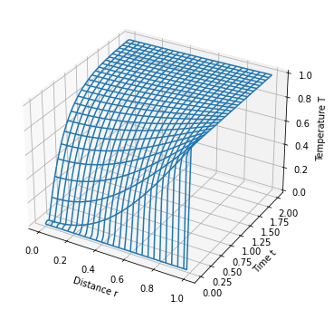
5.3.6. Cylindrical coordinates#
Suppressing the prime notation, for a cylindrical geometry the model specializes to
Expanding,
with auxiliary conditions
m = ConcreteModel()

m.r = ContinuousSet(bounds=(0,1))
m.t = ContinuousSet(bounds=(0,2))

m.T = Var(m.t, m.r)

m.dTdt   = DerivativeVar(m.T, wrt=m.t)
m.dTdr   = DerivativeVar(m.T, wrt=m.r)
m.d2Tdr2 = DerivativeVar(m.T, wrt=(m.r, m.r))

m.pde = Constraint(m.t, m.r, rule=lambda m, t, r: m.dTdt[t,r] == m.d2Tdr2[t,r] + (1/r)*m.dTdr[t,r]
        if r > 0 and r < 1 and t > 0 else Constraint.Skip)

m.ic  = Constraint(m.r, rule=lambda m, r:    m.T[0,r] == 0)
m.bc1 = Constraint(m.t, rule=lambda m, t:    m.T[t,1] == 1 if t > 0 else Constraint.Skip)
m.bc2 = Constraint(m.t, rule=lambda m, t: m.dTdr[t,0] == 0)

TransformationFactory('dae.finite_difference').apply_to(m, nfe=20, wrt=m.r, scheme='CENTRAL')
TransformationFactory('dae.finite_difference').apply_to(m, nfe=50, wrt=m.t, scheme='BACKWARD')
SolverFactory('ipopt').solve(m).write()

model_plot(m)
# ==========================================================
# = Solver Results                                         =
# ==========================================================
# ----------------------------------------------------------
#   Problem Information
# ----------------------------------------------------------
Problem:
- Lower bound: -inf
  Upper bound: inf
  Number of objectives: 1
  Number of constraints: 4060
  Number of variables: 4110
  Sense: unknown
# ----------------------------------------------------------
#   Solver Information
# ----------------------------------------------------------
Solver:
- Status: ok
  Message: Ipopt 3.13.4\x3a Optimal Solution Found
  Termination condition: optimal
  Id: 0
  Error rc: 0
  Time: 0.4122738838195801
# ----------------------------------------------------------
#   Solution Information
# ----------------------------------------------------------
Solution:
- number of solutions: 0
  number of solutions displayed: 0
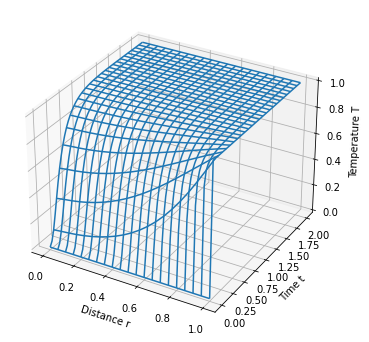
5.3.7. Spherical coordinates#
Suppressing the prime notation, for a cylindrical geometry the model specializes to
Expanding,
with auxiliary conditions
m = ConcreteModel()

m.r = ContinuousSet(bounds=(0,1))
m.t = ContinuousSet(bounds=(0,2))

m.T = Var(m.t, m.r)

m.dTdt   = DerivativeVar(m.T, wrt=m.t)
m.dTdr   = DerivativeVar(m.T, wrt=m.r)
m.d2Tdr2 = DerivativeVar(m.T, wrt=(m.r, m.r))

m.pde = Constraint(m.t, m.r, rule=lambda m, t, r: m.dTdt[t,r] == m.d2Tdr2[t,r] + (2/r)*m.dTdr[t,r]
        if r > 0 and r < 1 and t > 0 else Constraint.Skip)

m.ic  = Constraint(m.r, rule=lambda m, r:    m.T[0,r] == 0)
m.bc1 = Constraint(m.t, rule=lambda m, t:    m.T[t,1] == 1 if t > 0 else Constraint.Skip)
m.bc2 = Constraint(m.t, rule=lambda m, t: m.dTdr[t,0] == 0)

TransformationFactory('dae.finite_difference').apply_to(m, nfe=20, wrt=m.r, scheme='CENTRAL')
TransformationFactory('dae.finite_difference').apply_to(m, nfe=50, wrt=m.t, scheme='BACKWARD')
SolverFactory('ipopt').solve(m).write()

model_plot(m)
# ==========================================================
# = Solver Results                                         =
# ==========================================================
# ----------------------------------------------------------
#   Problem Information
# ----------------------------------------------------------
Problem:
- Lower bound: -inf
  Upper bound: inf
  Number of objectives: 1
  Number of constraints: 4060
  Number of variables: 4110
  Sense: unknown
# ----------------------------------------------------------
#   Solver Information
# ----------------------------------------------------------
Solver:
- Status: ok
  Message: Ipopt 3.13.4\x3a Optimal Solution Found
  Termination condition: optimal
  Id: 0
  Error rc: 0
  Time: 0.40662384033203125
# ----------------------------------------------------------
#   Solution Information
# ----------------------------------------------------------
Solution:
- number of solutions: 0
  number of solutions displayed: 0