Transportation Networks

3.1. Transportation Networks#

Keywords: transportation, assignment, cbc usage

This notebook demonstrates the solution of transportation network problems using Pyomo and GLPK. The problem description and data are adapted from Chapter 5 of Johannes Bisschop, “AIMMS Optimization Modeling”, AIMMS B. V., 2014.

3.1.1. Imports#

import shutil
import sys
import os.path

if not shutil.which("pyomo"):
    !pip install -q pyomo
    assert(shutil.which("pyomo"))

if not (shutil.which("cbc") or os.path.isfile("cbc")):
    if "google.colab" in sys.modules:
        !apt-get install -y -qq coinor-cbc
    else:
        try:
            !conda install -c conda-forge coincbc 
        except:
            pass

assert(shutil.which("cbc") or os.path.isfile("cbc"))
    
from pyomo.environ import *

3.1.2. Background#

The prototypical transportation problem deals with the distribution of a commodity from a set of sources to a set of destinations. The object is to minimize total transportation costs while satisfying constraints on the supplies available at each of the sources, and satisfying demand requirements at each of the destinations.

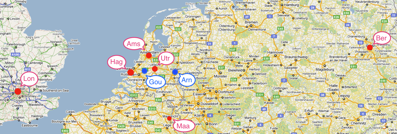
Here we illustrate the transportation problem using an example from Chapter 5 of Johannes Bisschop, “AIMMS Optimization Modeling”, Paragon Decision Sciences, 1999. In this example there are two factories and six customer sites located in 8 European cities as shown in the following map. The customer sites are labeled in red, the factories are labeled in blue.

Transportation costs between sources and destinations are given in units of €/ton of goods shipped, and list in the following table along with source capacity and demand requirements.

3.1.2.1. Table of transportation costs, customer demand, and available supplies#

Customer\Source	Arnhem [€/ton]	Gouda [€/ton]	Demand [tons]
London	-	2.5	125
Berlin	2.5	-	175
Maastricht	1.6	2.0	225
Amsterdam	1.4	1.0	250
Utrecht	0.8	1.0	225
The Hague	1.4	0.8	200
Supply [tons]	550 tons	700 tons

The situation can be modeled by links connecting a set nodes representing sources to a set of nodes representing customers.

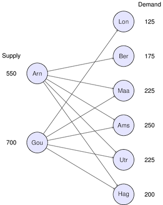
For each link we can have a parameter \(T[c,s]\) denoting the cost of shipping a ton of goods over the link. What we need to determine is the amount of goods to be shipped over each link, which we will represent as a non-negative decision variable \(x[c,s]\).

The problem objective is to minimize the total shipping cost to all customers from all sources.

\[\mbox{minimize:}\quad \mbox{Cost} = \sum_{c \in Customers}\sum_{s \in Sources} T[c,s] x[c,s]\]

Shipments from all sources can not exceed the manufacturing capacity of the source.

\[\sum_{c \in Customers} x[c,s] \leq \mbox{Supply}[s] \qquad \forall s \in Sources\]

Shipments to each customer must satisfy their demand.

\[\sum_{s\in Sources} x[c,s] = \mbox{Demand}[c] \qquad \forall c \in Customers\]

3.1.3. Pyomo model#

3.1.3.1. Data File#

Demand = {
   'Lon': 125,        # London
   'Ber': 175,        # Berlin
   'Maa': 225,        # Maastricht
   'Ams': 250,        # Amsterdam
   'Utr': 225,        # Utrecht
   'Hag': 200         # The Hague
}

Supply = {
   'Arn': 600,        # Arnhem
   'Gou': 650         # Gouda
}

T = {
    ('Lon', 'Arn'): 1000,
    ('Lon', 'Gou'): 2.5,
    ('Ber', 'Arn'): 2.5,
    ('Ber', 'Gou'): 1000,
    ('Maa', 'Arn'): 1.6,
    ('Maa', 'Gou'): 2.0,
    ('Ams', 'Arn'): 1.4,
    ('Ams', 'Gou'): 1.0,
    ('Utr', 'Arn'): 0.8,
    ('Utr', 'Gou'): 1.0,
    ('Hag', 'Arn'): 1.4,
    ('Hag', 'Gou'): 0.8
}

3.1.3.2. Model file#

# Step 0: Create an instance of the model
model = ConcreteModel()
model.dual = Suffix(direction=Suffix.IMPORT)

# Step 1: Define index sets
CUS = list(Demand.keys())
SRC = list(Supply.keys())

# Step 2: Define the decision 
model.x = Var(CUS, SRC, domain = NonNegativeReals)

# Step 3: Define Objective
@model.Objective(sense=minimize)
def cost(m):
    return sum([T[c,s]*model.x[c,s] for c in CUS for s in SRC])

# Step 4: Constraints
@model.Constraint(SRC)
def src(m, s):
    return sum([model.x[c,s] for c in CUS]) <= Supply[s]

@model.Constraint(CUS)
def dmd(m, c):
    return sum([model.x[c,s] for s in SRC]) == Demand[c]
    
results = SolverFactory('cbc').solve(model)
results.write()

# ==========================================================
# = Solver Results                                         =
# ==========================================================
# ----------------------------------------------------------
#   Problem Information
# ----------------------------------------------------------
Problem: 
- Name: unknown
  Lower bound: 1705.0
  Upper bound: 1705.0
  Number of objectives: 1
  Number of constraints: 9
  Number of variables: 13
  Number of nonzeros: 6
  Sense: minimize
# ----------------------------------------------------------
#   Solver Information
# ----------------------------------------------------------
Solver: 
- Status: ok
  User time: -1.0
  System time: 0.0
  Wallclock time: 0.0
  Termination condition: optimal
  Termination message: Model was solved to optimality (subject to tolerances), and an optimal solution is available.
  Statistics: 
    Branch and bound: 
      Number of bounded subproblems: None
      Number of created subproblems: None
    Black box: 
      Number of iterations: 1
  Error rc: 0
  Time: 0.026685237884521484
# ----------------------------------------------------------
#   Solution Information
# ----------------------------------------------------------
Solution: 
- number of solutions: 0
  number of solutions displayed: 0

3.1.4. Solution#

model.x.display()

x : Size=12, Index=x_index
    Key            : Lower : Value : Upper : Fixed : Stale : Domain
    ('Ams', 'Arn') :     0 :   0.0 :  None : False : False : NonNegativeReals
    ('Ams', 'Gou') :     0 : 250.0 :  None : False : False : NonNegativeReals
    ('Ber', 'Arn') :     0 : 175.0 :  None : False : False : NonNegativeReals
    ('Ber', 'Gou') :     0 :   0.0 :  None : False : False : NonNegativeReals
    ('Hag', 'Arn') :     0 :   0.0 :  None : False : False : NonNegativeReals
    ('Hag', 'Gou') :     0 : 200.0 :  None : False : False : NonNegativeReals
    ('Lon', 'Arn') :     0 :   0.0 :  None : False : False : NonNegativeReals
    ('Lon', 'Gou') :     0 : 125.0 :  None : False : False : NonNegativeReals
    ('Maa', 'Arn') :     0 : 225.0 :  None : False : False : NonNegativeReals
    ('Maa', 'Gou') :     0 :   0.0 :  None : False : False : NonNegativeReals
    ('Utr', 'Arn') :     0 : 200.0 :  None : False : False : NonNegativeReals
    ('Utr', 'Gou') :     0 :  25.0 :  None : False : False : NonNegativeReals

for c in CUS:
    for s in SRC:
        print(c, s, model.x[c,s]())

Lon Arn 0.0
Lon Gou 125.0
Ber Arn 175.0
Ber Gou 0.0
Maa Arn 225.0
Maa Gou 0.0
Ams Arn 0.0
Ams Gou 250.0
Utr Arn 200.0
Utr Gou 25.0
Hag Arn 0.0
Hag Gou 200.0

if 'ok' == str(results.Solver.status):
    print("Total Shipping Costs = ", model.cost())
    print("\nShipping Table:")
    for s in SRC:
        for c in CUS:
            if model.x[c,s]() > 0:
                print("Ship from ", s," to ", c, ":", model.x[c,s]())
else:
    print("No Valid Solution Found")

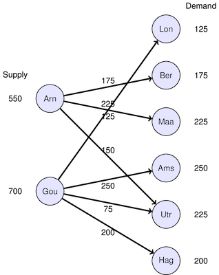
Total Shipping Costs =  1705.0

Shipping Table:
Ship from  Arn  to  Ber : 175.0
Ship from  Arn  to  Maa : 225.0
Ship from  Arn  to  Utr : 200.0
Ship from  Gou  to  Lon : 125.0
Ship from  Gou  to  Ams : 250.0
Ship from  Gou  to  Utr : 25.0
Ship from  Gou  to  Hag : 200.0

The solution has the interesting property that, with the exception of Utrecht, customers are served by just one source.

3.1.5. Sensitivity analysis#

3.1.5.1. Analysis by source#

if 'ok' == str(results.Solver.status):
    print("Source      Capacity   Shipped    Margin")
    for s in SRC:
        print(f"{s:10s}{Supply[s]:10.1f}{model.src[s]():10.1f}{model.dual[model.src[s]]:10.4f}")
else:
    print("No Valid Solution Found")

Source      Capacity   Shipped    Margin
Arn            600.0     600.0   -0.2000
Gou            650.0     600.0    0.0000

The ‘marginal’ values are telling us how much the total costs will be increased for each one ton increase in the available supply from each source. The optimization calculation says that only 650 tons of the 700 available from Gouda should used for a minimum cost solution, which rules out any further cost reductions by increasing the available supply. In fact, we could decrease the supply Gouda without any harm. The marginal value of Gouda is 0.

The source at Arnhem is a different matter. First, all 550 available tons are being used. Second, from the marginal value we see that the total transportations costs would be reduced by 0.2 Euros for each additional ton of supply.

The management conclusion we can draw is that there is excess supply available at Gouda which should, if feasible, me moved to Arnhem.

Now that’s a valuable piece of information!

3.1.5.2. Analysis by customer#

if 'ok' == str(results.Solver.status):    
    print("Customer      Demand   Shipped    Margin")
    for c in CUS:
        print(f"{c:10s}{Demand[c]:10.1f}{model.dmd[c]():10.1f}{model.dual[model.dmd[c]]:10.4f}")
else:
    print("No Valid Solution Found")

Customer      Demand   Shipped    Margin
Lon            125.0     125.0    2.5000
Ber            175.0     175.0    2.7000
Maa            225.0     225.0    1.8000
Ams            250.0     250.0    1.0000
Utr            225.0     225.0    1.0000
Hag            200.0     200.0    0.8000

Looking at the demand constraints, we see that all of the required demands have been met by the optimal solution.

The marginal values of these constraints indicate how much the total transportation costs will increase if there is an additional ton of demand at any of the locations. In particular, note that increasing the demand at Berlin will increase costs by 2.7 Euros per ton. This is actually greater than the list price for shipping to Berlin which is 2.5 Euros per ton. Why is this?

To see what’s going on, let’s resolve the problem with a one ton increase in the demand at Berlin.

We see the total cost has increased from 1715.0 to 1717.7 Euros, an increase of 2.7 Euros just as predicted by the marginal value assocated with the demand constraint for Berlin.

Now let’s look at the solution.

Here we see that increasing the demand in Berlin resulted in a number of other changes. This figure shows the changes shipments.

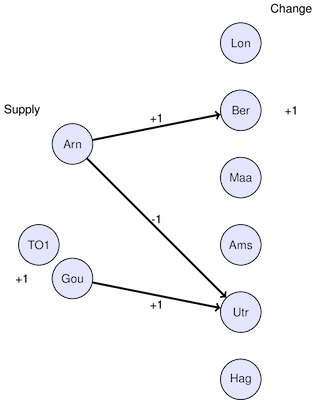
Shipments to Berlin increased from 175 to 176 tons, increasing costs for that link from 437.5 to 440.0, or a net increase of 2.5 Euros.
Since Arnhem is operating at full capacity, increasing the shipments from Arnhem to Berlin resulted in decreasing the shipments from Arhhem to Utrecht from 150 to 149 reducing those shipping costs from 120.0 to 119.2, a net decrease of 0.8 Euros.
To meet demand at Utrecht, shipments from Gouda to Utrecht had to increase from 75 to 76, increasing shipping costs by a net amount of 1.0 Euros.
The net effect on shipping costs is 2.5 - 0.8 + 1.0 = 2.7 Euros.

The important conclusion to draw is that when operating under optimal conditions, a change in demand or supply can have a ripple effect on the optimal solution that can only be measured through a proper sensitivity analysis.

3.1.6. Exercises#

Move 50 tons of supply capacity from Gouda to Arnhem, and repeat the sensitivity analysis. How has the situation improved? In practice, would you recommend this change, or would you propose something different?
What other business improvements would you recommend?