5.4. Diffusion with Adsorption in Polymers

5.4.1. References

• Paul, D. R. (1969). Effect of immobilizing adsorption on the diffusion time lag. Journal of Polymer Science Part A‐2: Polymer Physics, 7(10), 1811-1818. [pdf]

• Vieth, W. R., & Sladek, K. J. (1965). A model for diffusion in a glassy polymer. Journal of Colloid Science, 20(9), 1014-1033. [doi]

5.4.2. Model

Here we consider the diffusion of a small molecule into an immobile substrate with adsorption. Following the cited references:

\[\begin{split} \begin{align*} \frac{\partial (c + c_a)}{\partial t} & = D \frac{\partial^2 c}{\partial x^2} \\ \end{align*} \end{split}\]

Langmuir isotherm:

\[ \begin{align*} c_a & = \frac{q K c}{1 + K c} \end{align*} \]

After application of the chain rule:

\[\begin{split} \begin{align*} \left[1 + \frac{q K}{(1 + K c)^2}\right]\frac{\partial c}{\partial t} & = D \frac{\partial^2 c}{\partial x^2} \\ \end{align*} \end{split}\]

Initial conditions for \(c(t, x)\):

\[\begin{split} \begin{align*} c(0, x) & = 0 & 0 < x \leq L \\ \end{align*} \end{split}\]

Boundary conditions for \(c(t, x)\):

\[\begin{split} \begin{align*} c(t, 0) & = C_0 & t \geq 0 \\ c_x(t, L) & = 0 & t \geq 0 \\ \end{align*} \end{split}\]

Exercise 1: Verify the use of the chain rule. Generalize to an arbitrary isotherm \(c = f(c_a)\).

Exercise 2: Compare the dimensional and dimensionless implementations by finding values for dimensionless value of \(\alpha\) and surface concentration that reproduce the simulation results observed in dimensional model.

Exercise 3: Implement a Pyomo model as a DAE without using the chain rule.

Exercise 4: Replace the finite difference transformation on \(x\) with collocation. What (if any) practical advantages are associated with collocation?

Exercise 5: Revise the problem and model with a linear isotherm \(c_a = K c\), and use the solution concentration \(C_s\) to scale \(c(t, x)\). How many independent physical parameters exist for this problem? Find the analytical solution, and compare to a numerical solution found using Pyomo.DAE.

Exercise 6: Revise the dimensionless model for the Langmuir isotherm to use the solution concentraion \(C_s\) to scale \(c(x, t)\). How do the models compare? How many independent parameters exist for this problem? What physical or chemical interpretations can you assign to the dimensionless parameters appearing in the models?

Exercise 7: The Langmuir isotherm is an equilibrium relationship between absorption and desorption processes. The Langmuir isotherm assumes these processes are much faster than diffusion. Formulate the model for the case where absorption and desorption kinetics are on a time scale similar to the diffusion process.

5.4.3. Installations and Imports

import matplotlib.pyplot as plt
import numpy as np

import shutil
import sys
import os.path

if not shutil.which("pyomo"):
    !pip install -q pyomo
    assert(shutil.which("pyomo"))

if not (shutil.which("ipopt") or os.path.isfile("ipopt")):
    if "google.colab" in sys.modules:
        !wget -N -q "https://ampl.com/dl/open/ipopt/ipopt-linux64.zip"
        !unzip -o -q ipopt-linux64
    else:
        try:
            !conda install -c conda-forge ipopt 
        except:
            pass

assert(shutil.which("ipopt") or os.path.isfile("ipopt"))

5.4.4. Pyomo model

import pyomo.environ as pyo
import pyomo.dae as dae

# parameters
tf = 80
D = 2.68
L = 1.0
KL = 20000.0
Cs = 0.0025
qm = 1.0

m = pyo.ConcreteModel()

m.t = dae.ContinuousSet(bounds=(0, tf))
m.x = dae.ContinuousSet(bounds=(0, L))

m.c = pyo.Var(m.t, m.x)
m.dcdt = dae.DerivativeVar(m.c, wrt=m.t)
m.dcdx = dae.DerivativeVar(m.c, wrt=m.x)
m.d2cdx2 = dae.DerivativeVar(m.c, wrt=(m.x, m.x))

@m.Constraint(m.t, m.x)
def pde(m, t, x):
    return m.dcdt[t, x] * (1 + qm*KL/(1 + KL*m.c[t, x])** 2) == D * m.d2cdx2[t, x]

@m.Constraint(m.t)
def bc1(m, t):
    return m.c[t, 0] == Cs

@m.Constraint(m.t)
def bc2(m, t):
    return m.dcdx[t, L] == 0

@m.Constraint(m.x)
def ic(m, x):
    if x == 0:
        return pyo.Constraint.Skip
    return m.c[0, x] == 0.0

# transform and solve
pyo.TransformationFactory('dae.finite_difference').apply_to(m, wrt=m.x, nfe=40)
pyo.TransformationFactory('dae.finite_difference').apply_to(m, wrt=m.t, nfe=40)
pyo.SolverFactory('ipopt').solve(m).write()

# ==========================================================
# = Solver Results                                         =
# ==========================================================
# ----------------------------------------------------------
#   Problem Information
# ----------------------------------------------------------
Problem: 
- Lower bound: -inf
  Upper bound: inf
  Number of objectives: 1
  Number of constraints: 6682
  Number of variables: 6683
  Sense: unknown
# ----------------------------------------------------------
#   Solver Information
# ----------------------------------------------------------
Solver: 
- Status: ok
  Message: Ipopt 3.13.4\x3a Optimal Solution Found
  Termination condition: optimal
  Id: 0
  Error rc: 0
  Time: 1.7579870223999023
# ----------------------------------------------------------
#   Solution Information
# ----------------------------------------------------------
Solution: 
- number of solutions: 0
  number of solutions displayed: 0

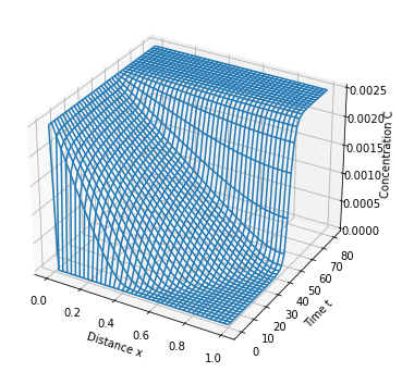
5.4.5. Visualization

def model_plot(m):
    t = sorted(m.t)
    x = sorted(m.x)

    xgrid = np.zeros((len(t), len(x)))
    tgrid = np.zeros((len(t), len(x)))
    cgrid = np.zeros((len(t), len(x)))

    for i in range(0, len(t)):
        for j in range(0, len(x)):
            xgrid[i,j] = x[j]
            tgrid[i,j] = t[i]
            cgrid[i,j] = m.c[t[i], x[j]].value

    fig = plt.figure(figsize=(10,6))
    ax = fig.add_subplot(1, 1, 1, projection='3d')
    ax.set_xlabel('Distance x')
    ax.set_ylabel('Time t')
    ax.set_zlabel('Concentration C')
    p = ax.plot_wireframe(xgrid, tgrid, cgrid)

# visualization
model_plot(m)

5.4.6. Dimensional analysis

\[\begin{split} \begin{align*} x & = L x' \\ c & = C c' \\ t & = T t' \\ \end{align*} \end{split}\]

\[\begin{split} \begin{align*} \left[1 + \frac{q K}{(1 + K C c')^2}\right]\frac{\partial c'}{\partial t'} & = \frac{TD}{L^2} \frac{\partial^2 c'}{\partial x'^2} \\ \end{align*} \end{split}\]

Assuming \(L\) is determined by the experimental apparatus, choose

\[\begin{split} \begin{align*} T & = \frac{L^2}{D} \\ C & = \frac{1}{K} \\ \end{align*} \end{split}\]

which results in a one parameter model

\[\begin{split} \begin{align*} \left[1 + \frac{\alpha}{(1 + c')^2}\right]\frac{\partial c'}{\partial t'} & = \frac{\partial^2 c'}{\partial x'^2} \\ \end{align*} \end{split}\]

where \(\alpha = q K\) represents a dimensionless capacity of the substrate to absorb the diffusing molecule.

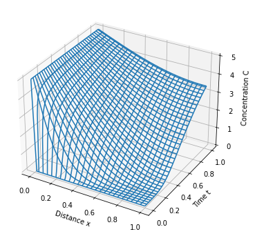
5.4.7. Dimensionless Pyomo model

import pyomo.environ as pyo
import pyomo.dae as dae

# parameters
tf = 1.00
Cs = 5.0
alpha = 5.0

m = pyo.ConcreteModel()

m.t = dae.ContinuousSet(bounds=(0, tf))
m.x = dae.ContinuousSet(bounds=(0, 1))

m.c = pyo.Var(m.t, m.x)
m.s = pyo.Var(m.t, m.x)

m.dcdt = dae.DerivativeVar(m.c, wrt=m.t)
m.dcdx = dae.DerivativeVar(m.c, wrt=m.x)
m.d2cdx2 = dae.DerivativeVar(m.c, wrt=(m.x, m.x))

@m.Constraint(m.t, m.x)
def pde(m, t, x):
    return m.dcdt[t, x] * (1 + alpha/(1 + m.c[t, x])** 2) == m.d2cdx2[t, x]

@m.Constraint(m.t)
def bc1(m, t):
    return m.c[t, 0] == Cs

@m.Constraint(m.t)
def bc2(m, t):
    return m.dcdx[t, 1] == 0

@m.Constraint(m.x)
def ic(m, x):
    if (x == 0) or (x == 1):
        return pyo.Constraint.Skip
    return m.c[0, x] == 0.0

# transform and solve
pyo.TransformationFactory('dae.finite_difference').apply_to(m, wrt=m.x, nfe=50)
pyo.TransformationFactory('dae.finite_difference').apply_to(m, wrt=m.t, nfe=100)
pyo.SolverFactory('ipopt').solve(m).write()

model_plot(m)

# ==========================================================
# = Solver Results                                         =
# ==========================================================
# ----------------------------------------------------------
#   Problem Information
# ----------------------------------------------------------
Problem: 
- Lower bound: -inf
  Upper bound: inf
  Number of objectives: 1
  Number of constraints: 20501
  Number of variables: 20503
  Sense: unknown
# ----------------------------------------------------------
#   Solver Information
# ----------------------------------------------------------
Solver: 
- Status: ok
  Message: Ipopt 3.13.4\x3a Optimal Solution Found
  Termination condition: optimal
  Id: 0
  Error rc: 0
  Time: 3.6713459491729736
# ----------------------------------------------------------
#   Solution Information
# ----------------------------------------------------------
Solution: 
- number of solutions: 0
  number of solutions displayed: 0