2.6. Model Predictive Control of a Double Integrator

Keywords: model predictive control, cbc usage

2.6.1. Imports

%matplotlib inline
from itertools import chain
import logging
from mpl_toolkits.mplot3d import Axes3D  
import matplotlib.pyplot as plt
import math
import numpy as np
import random
from scipy.interpolate import interp2d
from scipy.integrate import odeint

import shutil
import sys
import os.path

if not shutil.which("pyomo"):
    !pip install -q pyomo
    assert(shutil.which("pyomo"))

if not (shutil.which("cbc") or os.path.isfile("cbc")):
    if "google.colab" in sys.modules:
        !apt-get install -y -qq coinor-cbc
    else:
        try:
            !conda install -c conda-forge coincbc 
        except:
            pass

assert(shutil.which("cbc") or os.path.isfile("cbc"))

from pyomo.environ import *

2.6.2. Model

The double integrator model is a canonical second order linear system often used to demonstrate control principles. A typical example is Newton’s second law where a frictionless mass \(m\) is subject to external forces in one dimension

\[\begin{split} \begin{align*} m \frac{d^2x}{dt^2} & = f(t) \\ \end{align*} \end{split}\]

where \(x\) is position and \(f(t)\) is the applied force. It is also reasonably approximates the response of a motor to torque inputs, to a ball moving on a beam that can be tilted, and other mechanical systems. Here we consider a case where the control input \(f(t)\) and the position \(x(t)\) are both bounded in magnitude.

\[\begin{split} \begin{align*} | f(t) | & \leq F \\ | x(t) | & \leq L \\ \end{align*} \end{split}\]

Introducing scaling rules

\[ \begin{align*} y = \frac{x}{L} \qquad u = \frac{f}{F} \qquad \tau = \frac{t}{T} \end{align*} \]

results in the equation

\[\frac{m L}{T^2F} \frac{d^2y}{d\tau^2} = u\]

Choosing the time scale \(T\) as

\[T = \sqrt{\frac{mL}{F}}\]

reduces the control problem to a dimensionless form

\[\begin{split} \begin{align*} \frac{d^2y}{d\tau^2} & = u \\ \end{align*} \end{split}\]

subject to constraints

\[\begin{split} \begin{align*} |u(\tau)| & \leq 1 \qquad \forall \tau \in [0, 1]\\ |y(\tau)| & \leq 1 \qquad \forall \tau \in [0, 1] \end{align*} \end{split}\]

A variety of control problems that can be formulated from this simple model. Here we consider the problem of determining the range of possible initial conditions \(y(0)\) and \(\dot{y}(0)\) that can be steered back to a steady position at the origin (i.e., \(y = 0\) and \(\dot{y} = 0\)) without violating the constraints on position or applied control action. For the ball-on-beam experiment, this would correspond to finding initial conditions for the position and velocity of the ball that can be steered back to a steady position at the center of the beam without falling off in the meanwhile.

2.6.3. Discrete time approximation

In order to directly construct an optimization model, here we will consider a discrete-time approximation to the double integrator model. We will assume values of \(u(\tau)\) are fixed at discrete points in time \(\tau_k = kh\) where \(k = 0, 1, \ldots, N\) and \(h = \frac{T}{N}\) is the sampling time. The control input is held constant between these sample points.

Using the notation \(x_1 = y\) and \(x_2= \dot{y}\) we have

\[\begin{split} \begin{align*} \frac{dx_1}{d\tau} & = x_2\\ \frac{dx_2}{d\tau} & = u \end{align*} \end{split}\]

Because \(u\) is constant between sample instants, integrating the second equation gives

\[x_2(\tau_k + h) = x_2(\tau_k) + h u(\tau_k)\]

Substituting and integrating the first equation then yields the pair of equations

\[\begin{split} \begin{align*} x_1(\tau_k + h) & = x_1(\tau_k) + h x_2(\tau_k) + \frac{h^2}{2} u(\tau_k)\\ x_2(\tau_k + h) & = x_2(\tau_k) + h u(\tau_k) \end{align*} \end{split}\]

This discretization gives

\[\begin{split} \begin{align*} \underbrace{\begin{bmatrix}x_1(\tau_k+h) \\ x_2(\tau_k+h)\end{bmatrix}}_{x(\tau_{k+1})} & = \underbrace{\begin{bmatrix}1 & h \\ 0 & 1 \end{bmatrix}}_A \underbrace{\begin{bmatrix}x_1(\tau_k) \\ x_2(\tau_k)\end{bmatrix}}_{x(\tau_k)} + \underbrace{\begin{bmatrix}\frac{h^2}{2} \\ h \end{bmatrix}}_B u(\tau_k) \\ y(\tau_k) & = \underbrace{\begin{bmatrix} 1 & 0 \end{bmatrix}}_C \underbrace{\begin{bmatrix}x_1(\tau_k) \\ x_2(\tau_k)\end{bmatrix}}_{x(\tau_k)} \end{align*} \end{split}\]

where \(y(\tau_k)\) corresponds to position. The constraints are

\[\begin{split} \begin{align*} | u(\tau_k) | & \leq 1 \qquad \forall\ k=0, 1, \ldots, N \\ | y(\tau_k) | & \leq 1 \qquad \forall\ k=0, 1, \ldots, N \end{align*} \end{split}\]

For the purposes here, we will neglect constaints on the dynamics during the periods between sample points. Any issues with intersample dynamics can be addressed by increasing the number of sample points.

2.6.4. Model predictive control

Given values of the state variables \(x_1(\tau_0)\) and \(x_2(\tau_0)\) and sampling time \(h = \frac{T}{N}\) the computational task is to find a control policy \(u(\tau_k), u(\tau_{k+1}), \ldots, u(\tau_{k+N-1})\) that steers the state to the origin at \(t_{k+N}\). The model equations are

\[\begin{split} \begin{align*} x_1(\tau_{k+1}) & = x_1(\tau_k) + h x_2(\tau_k) + \frac{h^2}{2} u(\tau_k)\\ x_2(\tau_{k + 1}) & = x_2(\tau_k) + h u(\tau_k) \\ y(\tau_k) & = x_1(\tau_k) \end{align*} \end{split}\]

for \(k = 0, 1, \ldots, N-1\), subject to final conditions

\[\begin{split} \begin{align*} x_1(\tau_{k+N}) & = 0 \\ x_2(\tau_{k+N}) & = 0 \end{align*} \end{split}\]

and path constraints

\[\begin{split} \begin{align*} |u(\tau_k)| & \leq 1 \qquad \forall k = 0, 1, 2, \ldots, N-1 \\ |y(\tau_k)| & \leq 1 \qquad \forall k = 0, 1, 2, \ldots, N-1 \end{align*} \end{split}\]

The path constraints need to be recast for the purposes of linear optimization. Here we introduce additional decision variables

\[\begin{split} \begin{align*} u(\tau_k) & = u^+(\tau_k) - u^-(\tau_k) \\ y(\tau_k) & = y^+(\tau_k) - y^-(\tau_k) \end{align*} \end{split}\]

where

\[\begin{split} \begin{align*} 0 \leq u^+(\tau_k), u^-(\tau_k) & \leq 1 \\ 0 \leq y^+(\tau_k), y^-(\tau_k) & \leq 1 \end{align*} \end{split}\]

The objective function is then to minimize

\[\min \sum_{k=0}^N\gamma \left[u^+(\tau_k)+ u^-(\tau_k)\right] + (1-\gamma) \left[y^+(\tau_k) + y^-(\tau_k)\right]\]

for a choice of \( 0 < \gamma < 1\) that represents a desired tradeoff between path constraints on \(u(\tau_k)\) and \(y(\tau_k)\).

def mpc_double_integrator(N=2, h=1):
    m = ConcreteModel()
    m.states = RangeSet(1, 2)
    m.k = RangeSet(0, N)
    
    m.h = Param(initialize=h, mutable=True)
    m.ic = Param(m.states, initialize={1:0.5, 2:0.5}, mutable=True)
    m.gamma = Param(default=0.5, mutable=True)
    
    m.x = Var(m.states, m.k)
    m.icfix = Constraint(m.states, rule = lambda m, i: m.x[i,0] == m.ic[i])
    m.x[1,N].fix(0)
    m.x[2,N].fix(0)
    
    m.u = Var(m.k, bounds=(-1, 1))
    m.upos = Var(m.k, bounds=(0, 1))
    m.uneg = Var(m.k, bounds=(0, 1))
    m.usum = Constraint(m.k, rule = lambda m, k: m.u[k] == m.upos[k] - m.uneg[k])   
  
    m.y = Var(m.k, bounds=(-1, 1))
    m.ypos = Var(m.k, bounds=(0, 1))
    m.yneg = Var(m.k, bounds=(0, 1))
    m.ysum = Constraint(m.k, rule = lambda m, k: m.y[k] == m.ypos[k] - m.yneg[k])

    m.x1_update = Constraint(m.k, rule = lambda m, k:
           m.x[1,k+1] == m.x[1,k] + m.h*m.x[2,k] + m.h**2*m.u[k]/2 if k < N else Constraint.Skip)
    m.x2_update = Constraint(m.k, rule = lambda m, k:
           m.x[2,k+1] == m.x[2,k] + m.h*m.u[k] if k < N else Constraint.Skip)
    m.y_output = Constraint(m.k, rule = lambda m, k: m.y[k] == m.x[1,k])
    
    m.uobj = m.gamma*sum(m.upos[k] + m.uneg[k] for k in m.k)
    m.yobj = (1-m.gamma)*sum(m.ypos[k] + m.yneg[k] for k in m.k)
    m.obj = Objective(expr = m.uobj + m.yobj, sense=minimize)
    
    return m

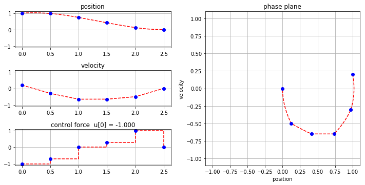
2.6.5. Visualization

def plot_results(m):
    results = SolverFactory('cbc').solve(m)
    if str(results.solver.termination_condition) != "optimal":
        print(results.solver.termination_condition)
        return
    
    # solution data at sample times
    h = m.h()
    K = np.array([k for k in m.k])  
    u = [m.u[k]() for k in K]
    y = [m.y[k]() for k in K]
    v = [m.x[2,k]() for k in K]
    
    # interpolate between sample times
    t = np.linspace(0, h) 
    tp = [_ for _ in chain.from_iterable(k*h + t for k in K[:-1])]
    up = [_ for _ in chain.from_iterable(u[k] + t*0 for k in K[:-1])]
    yp = [_ for _ in chain.from_iterable(y[k] + t*(v[k] + t*u[k]/2) for k in K[:-1])]
    vp = [_ for _ in chain.from_iterable(v[k] + t*u[k] for k in K[:-1])]

    fig = plt.figure(figsize=(10,5))
    
    ax1 = fig.add_subplot(3, 2, 1)
    ax1.plot(tp, yp, 'r--', h*K, y, 'bo')
    ax1.set_title('position')

    ax2 = fig.add_subplot(3, 2, 3)
    ax2.plot(tp, vp, 'r--', h*K, v, 'bo')
    ax2.set_title('velocity')

    ax3 = fig.add_subplot(3, 2, 5)
    ax3.plot(np.append(tp, K[-1]*h), np.append(up, u[-1]), 'r--', h*K, u, 'bo')
    ax3.set_title('control force  u[0] = {0:<6.3f}'.format(u[0]))

    ax4 = fig.add_subplot(1, 2, 2)
    ax4.plot(yp, vp, 'r--', y, v, 'bo')
    ax4.set_xlim([-1.1, 1.1])
    ax4.set_aspect('equal', 'box')
    ax4.set_title('phase plane')
    ax4.set_xlabel('position')
    ax4.set_ylabel('velocity')
    
    for ax in [ax1, ax2, ax3, ax4]:
        ax.set_ylim(-1.1, 1.1)
        ax.grid(True)
    fig.tight_layout()

model = mpc_double_integrator(5, 0.5)
model.ic[1] = 1.0
model.ic[2] = 0.2

SolverFactory('cbc').solve(model)
plot_results(model)

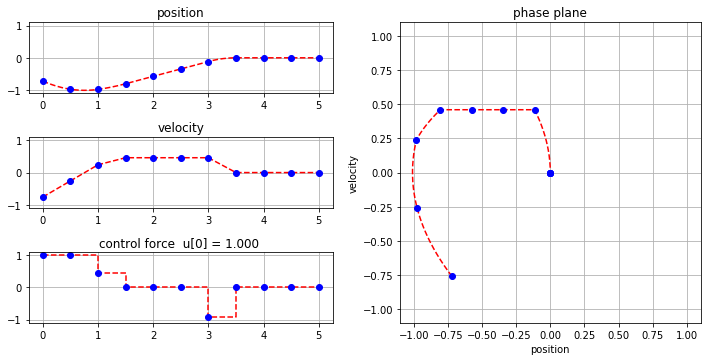
2.6.6. Interactive use

2.6.6.1. Google Colaboratory

When run in Google Colaboratory, the following cell opens a GUI form that can be used interact with the model described above.

#@title Interactive { run: "auto" }

N = 10 #@param {type: "slider", min:1, max:20, step:1}
h = 0.5 #@param {type:"slider", min:0, max:1, step:0.01}
gamma = 0.54 #@param {type:"slider", min:0, max:1, step:0.01}
x_initial = -0.72 #@param {type:"slider", min:-1, max:1, step:0.01}
v_initial = -0.76 #@param {type:"slider", min:-1, max:1, step:0.01}

model = mpc_double_integrator(N, h)
model.gamma = gamma
model.ic[1] = x_initial
model.ic[2] = v_initial

SolverFactory('cbc').solve(model)
plot_results(model)

2.6.7. Model predictive control as a feedback controller

Model Predictive Control is a control strategy that uses open-loop optimal control calculations to implement feedback control. The concept behind MPC is to continually update an optimal control policy as new sensor information becomes available. Then at each point in time, the manipulated variable is set to the first value in the updated control policy.

For low dimensional systems like the double integrator, it is possible to compute optimal control policies for all feasible initial conditions. The control input is then the first value of the resulting control policy. The result can be written as a function

\[u(\tau) = mpc(x_1(\tau), x_2(\tau))\]

The following cell demonstrates the calculation of the control policy as a function initial conditions. The result will be a matrix \(U\) of control values computed for 2D grid of values for initial position and velocity.

# turn off pyomo warnings
logging.getLogger('pyomo.core').setLevel(logging.ERROR)

model = mpc_double_integrator(10)
model.h = 0.5
model.gamma = 0.4

def fun(y, v):
    u = 0*y
    for i in range(0, len(y)):
        model.ic[1] = y[i]
        model.ic[2] = v[i]
        results = SolverFactory('cbc').solve(model)
        if str(results.solver.termination_condition) == 'optimal':
            u[i] = model.u[0]()
        else:
            u[i] = None
    return u

fig = plt.figure(figsize=(10,8))
ax = fig.add_subplot(111, projection='3d')

y = v = np.arange(-0.7, 0.7, 0.1)
Y, V = np.meshgrid(y, v)
u = np.array(fun(np.ravel(Y), np.ravel(V)))
U = u.reshape(V.shape)

ax.plot_surface(V, Y, U)
ax.set_xlabel('initial velocity')
ax.set_ylabel('initial position')
ax.set_zlabel('control force')

Text(0.5, 0, 'control force')

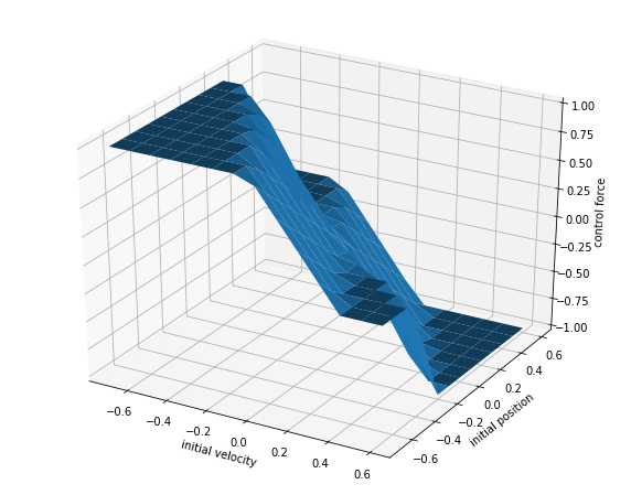
The results of the MPC calculation are recorded in a matrix \(U\). In the next cell we create 2D interpolation object that will be used for simulation of the closed-loop system.

mpc = interp2d(Y, V, U)

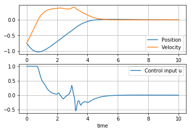
Next we perform a continuous time simulation where the interpolator is used for feedback control. Compare this result to one obtained above for same initial condition.

def mpc_sim(x, t):
    y, v = x
    return [v, mpc(y,v)]

t = np.linspace(0, 10, 200)
x = odeint(mpc_sim, [-0.75, -0.75], t)

plt.subplot(2,1,1)
plt.plot(t,x)
plt.xlabel('time')
plt.legend(['Position', 'Velocity'])
plt.grid(True)

plt.subplot(2,1,2)
plt.plot(t, [mpc(x1, x2) for x1,x2 in x])
plt.xlabel('time')
plt.legend(['Control input u'])
plt.grid(True)