8.5. MAD Portfolio Optimization

Keywords: glpk usage, portfolio optimization, value at risk, stock price data

8.5.1. Imports

%matplotlib inline

import matplotlib.dates as mdates
import matplotlib.pyplot as plt
import numpy as np
import pandas as pd
import random
import scipy.stats as stats

import shutil
import sys
import os.path

if not shutil.which("pyomo"):
    !pip install -q pyomo
    assert(shutil.which("pyomo"))

if not (shutil.which("glpsol") or os.path.isfile("glpsol")):
    if "google.colab" in sys.modules:
        !apt-get install -y -qq glpk-utils
    else:
        try:
            !conda install -c conda-forge glpk 
        except:
            pass

assert(shutil.which("glpsol") or os.path.isfile("glpsol"))

from pyomo.environ import *

8.5.2. Investment objectives

• Maximize returns

• Reduce Risk through diversification

8.5.3. Why diversify?

Investment portfolios are collections of investments that are managed for overall investment return. Compared to investing all of your capital into a single asset, maintaining a portfolio of investments allows you to manage risk through diversification.

8.5.3.1. Reduce risk through law of large numbers

Suppose there are a set of independent investment opportunities that will pay back between 0 and 300% of your original investment, and that all outcomes in that range are equally likely. You have $100,000 to invest. Should you put it all in one opportunity? Or should you spread it around?

Here we simulate the outcomes of 1000 trials where we place all the money into a single investment of $100,000.

W0 = 100000.00

Ntrials = 10000
Profit = list()
for n in range(0, Ntrials):
    W1 = W0*random.uniform(0,3.00)
    Profit.append(W1 - W0)

plt.figure(figsize=(10, 4))
plt.hist(Profit, bins=100)
plt.xlim(-100000, 200000)
plt.xlabel('Profit')
plt.ylabel('Frequency')

print('Average Profit = ${:.0f}'.format(np.mean(Profit)))

Average Profit = $50737

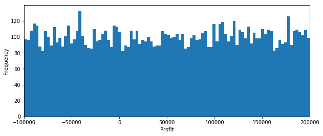
As you would expect, about 1/3 of the time there is a loss, and about 2/3 of the time there is a profit. In the extreme we can lose all of our invested capital. Is this an acceptable investment outcome?

Now let’s see if what happens if we diversify our investment. We’ll assume the investment outcomes have exactly the same probabilities. The only difference is that instead of one big investment of \\(100,000, we'll break our capital into 5 smaller sized investments of \\\)20,000 each. We’ll calculate the probability distribution of outcomes.

W0 = 100000.00

Ntrials = 10000
Ninvestments = 5

Profit = list()
for n in range(0,Ntrials):
    W1 = sum([(W0/Ninvestments)*random.uniform(0,3.00) for _ in range(0,Ninvestments)])
    Profit.append(W1-W0)

plt.figure(figsize=(10, 4))
plt.hist(Profit, bins=100)
plt.xlim(-100000, 200000)
plt.xlabel('Profit')
plt.ylabel('Frequency')

print('Average Profit = ${:.0f}'.format(np.mean(Profit)))

Average Profit = $50042

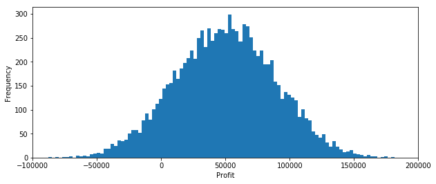
What we observe is that even a small amount of diversification can dramatically reduce the downside risk of experiencing a loss. We also see the upside potential has been reduced. What hasn’t changed is the that average profit remains at $50,000. Whether or not the loss of upside potential in order to reduce downside risk is an acceptable tradeoff depends on your individual attitude towards risk.

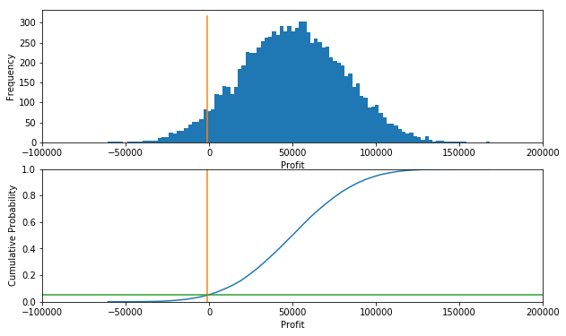
8.5.3.2. Value at risk (VaR)

Value at risk (VaR) is a measure of investment risk. Given a histogram of possible outcomes for the profit of a portfolio, VaR corresponds to negative value of the 5th percentile. That is, 5% of all outcomes would have a lower outcome, and 95% would have a larger outcome.

The conditional value at risk (also called the expected shortfall (ES), average value at risk (aVaR), and the expected tail loss (ETL)) is the negative of the average value of the lowest 5% of outcomes.

The following cell provides an interactive demonstration. Use the slider to determine how to break up the total available capital into a number of smaller investments in order to reduce the value at risk to an acceptable (to you) level. If you can accept only a 5% probability of a loss in your portfolio, how many individual investments would be needed?

#@title Value at Risk (VaR) Demo { run: "auto", vertical-output: true }
Ninvestments = 8 #@param {type:"slider", min:1, max:20, step:1}

from statsmodels.distributions import ECDF

W0 = 100000.00
Ntrials = 10000

def sim(Ninvestments = 5):

    Profit = list()
    for n in range(0, Ntrials):
        W1 = sum([(W0/Ninvestments)*random.uniform(0,3.00) for _ in range(0,Ninvestments)])
        Profit.append(W1-W0)
        
    print('Average Profit = ${:.0f}'.format(np.mean(Profit)).replace('$-','-$'))

    VaR = -sorted(Profit)[int(0.05*Ntrials)]
    print('Value at Risk (95%) = ${:.0f}'.format(VaR).replace('$-','-$'))
    
    cVaR = -sum(sorted(Profit)[0:int(0.05*Ntrials)])/(0.05*Ntrials)
    print('Conditional Value at Risk (95%) = ${:.0f}'.format(cVaR).replace('$-','-$'))

    plt.figure(figsize=(10,6))
    plt.subplot(2, 1, 1)
    plt.hist(Profit, bins=100)
    plt.xlim(-100000, 200000)
    plt.plot([-VaR, -VaR], plt.ylim())
    plt.xlabel('Profit')
    plt.ylabel('Frequency')

    plt.subplot(2, 1, 2)
    ecdf = ECDF(Profit)
    x = np.linspace(min(Profit), max(Profit))
    plt.plot(x, ecdf(x))
    plt.xlim(-100000, 200000)
    plt.ylim(0,1)
    plt.plot([-VaR, -VaR], plt.ylim())
    plt.plot(plt.xlim(), [0.05, 0.05])
    plt.xlabel('Profit')
    plt.ylabel('Cumulative Probability');
    
sim(Ninvestments)

Average Profit = $49825
Value at Risk (95%) = $1004
Conditional Value at Risk (95%) = $13011

8.5.4. Import historical stock price data

S_hist = pd.read_csv('data/Historical_Adjusted_Close.csv', index_col=0)

S_hist.dropna(axis=1, how='any', inplace=True)
S_hist.index = pd.DatetimeIndex(S_hist.index)

portfolio = list(S_hist.columns)
print(portfolio)
S_hist.tail()

['AAPL', 'AXP', 'BA', 'CAT', 'CSCO', 'CVX', 'DIS', 'GE', 'HD', 'IBM', 'INTC', 'JNJ', 'JPM', 'KO', 'MCD', 'MMM', 'MRK', 'MSFT', 'NKE', 'PFE', 'PG', 'T', 'TRV', 'UNH', 'UTX', 'VZ', 'WMT', 'XOM']

	AAPL	AXP	BA	CAT	CSCO	CVX	DIS	GE	HD	IBM	...	NKE	PFE	PG	T	TRV	UNH	UTX	VZ	WMT	XOM
2019-05-24	178.97	119.51	354.90	122.90	54.37	118.71	132.79	9.45	193.59	132.28	...	81.9263	41.95	106.69	32.27	147.94	247.63	131.40	59.32	102.67	74.10
2019-05-28	178.23	118.17	354.88	121.59	53.93	118.31	132.62	9.36	191.55	130.46	...	80.9691	41.90	104.46	31.93	146.28	242.06	129.92	58.73	102.42	72.61
2019-05-29	177.38	117.01	348.80	121.48	53.18	116.77	131.57	9.37	189.99	129.69	...	78.6457	41.72	104.19	31.91	145.07	242.40	129.47	58.18	102.12	72.16
2019-05-30	178.30	116.74	349.87	121.84	53.57	115.38	132.20	9.47	191.08	129.57	...	79.0346	41.90	105.33	31.86	145.73	243.50	128.40	56.83	102.19	71.97
2019-05-31	175.07	114.71	341.61	119.81	52.03	113.85	132.04	9.44	189.85	126.99	...	77.1400	41.52	102.91	30.58	145.57	241.80	126.30	54.35	101.44	70.77

5 rows × 28 columns

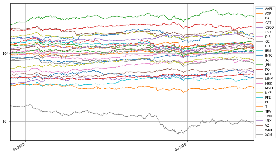
8.5.5. Select a recent subperiod of the historical data

nYears = 1.5
start = S_hist.index[-int(nYears*252)]
end = S_hist.index[-1]

print('Start Date:', start)
print('  End Date:', end)

S = S_hist.loc[start:end]
S.head()

Start Date: 2017-11-28 00:00:00
  End Date: 2019-05-31 00:00:00

	AAPL	AXP	BA	CAT	CSCO	CVX	DIS	GE	HD	IBM	...	NKE	PFE	PG	T	TRV	UNH	UTX	VZ	WMT	XOM
2017-11-28	169.1244	93.2036	259.9291	134.2662	36.0972	109.9599	100.9739	17.0878	170.5630	142.4311	...	58.4100	34.0208	85.0389	32.3601	128.5122	211.7681	113.8682	45.6521	93.0304	76.6965
2017-11-29	165.6162	94.4949	261.1997	133.3678	35.8580	110.6492	102.7608	17.1528	172.0796	143.4400	...	59.1746	34.3624	85.0199	33.3286	129.9808	218.3718	114.3035	46.6620	93.7899	77.2599
2017-11-30	167.9322	95.5807	268.4741	136.3528	35.6858	112.3583	102.3507	16.9765	174.5747	143.8323	...	59.2335	34.4099	85.6001	33.2372	130.9857	224.2896	117.4862	47.5878	93.4726	78.2178
2017-12-01	167.1504	95.7274	263.2171	136.7102	35.9728	112.8493	102.7706	16.5959	175.1572	144.5703	...	58.9001	34.4953	85.9521	33.3468	131.6040	222.9232	116.1996	47.9244	93.5880	78.3775
2017-12-04	165.9289	96.4415	269.6089	136.6909	36.0876	114.1052	107.6235	16.6609	179.5065	146.1584	...	59.1165	34.2201	86.9509	34.0503	131.7489	217.6544	116.1222	48.3639	93.2611	78.4808

5 rows × 28 columns

fig, ax = plt.subplots(figsize=(14,9))
S.plot(ax=ax, logy=True)

ax.xaxis.set_major_locator(mdates.YearLocator())
ax.xaxis.set_major_formatter(mdates.DateFormatter('%m-%Y'))
plt.legend(loc='center left', bbox_to_anchor=(1.0, 0.5))
plt.grid(True)

8.5.6. Return on a portfolio

Given a portfolio with value \(W_t\) at time \(t\), return on the portfolio at \(t_{t +\delta t}\) is defined as

\[ \begin{align*} r_{t + \delta t} & = \frac{W_{t + \delta t} - W_{t}}{W_{t}} \end{align*} \]

For the period from \([t, t+\delta t)\) we assume there are \(n_{j,t}\) shares of asset \(j\) with a starting value of \(S_{j,t}\) per share. The initial and final values of the portfolio are then

\[\begin{split} \begin{align*} W_t & = \sum_{j=1}^J n_{j,t}S_{j,t} \\ W_{t+\delta t} & = \sum_{j=1}^J n_{j,t}S_{j,t + \delta t} \end{align*} \end{split}\]

The return of the portfolio is given by

\[\begin{split} \begin{align*} r_{t+\delta t} & = \frac{W_{t + \delta t} - W_{t}}{W_{t}} \\ & = \frac{\sum_{j=1}^Jn_{j,t}S_{j,t+\delta t} - \sum_{j=1}^J n_{j,t}S_{j,t}}{W_{t}} \\ & = \frac{\sum_{j=1}^J n_{j,t}S_{j,t}r_{j, t+\delta t}}{W_{t}} \\ & = \sum_{j=1}^J \frac{n_{j,t}S_{j,t}}{W_{t}} r_{j, t+\delta t} \end{align*} \end{split}\]

where \(r_{j,t+\delta t}\) is the return on asset \(j\) at time \(t+\delta t\).

Defining \(W_{j,t} = n_{j,t}S_{j,t}\) as the wealth invested in asset \(j\) at time \(t\), then \(w_{j,t} = n_{j,t}S_{j,t}/W_{t}\) is the fraction of total wealth invested in asset \(j\) at time \(t\). The portfolio return is then given by

\[ \begin{align*} r_{t+\delta t} & = \sum_{j=1}^J w_{j,t} r_{j, t+\delta t} \end{align*} \]

on a single interval extending from \(t\) to \(t + \delta t\).

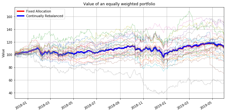
8.5.6.1. Equally weighted portfolio

An equally weighted portfolio allocates an equal amount of capital to each component of the portfolio. The allocation can be done once and held fixed thereafter, or could be reallocated periodically as asset prices change in relation to one another.

8.5.6.1.1. Constant fixed allocation

If the initial allocation among \(J\) assets takes place at \(t=0\), then

\[w_{j,0} = \frac{1}{J} = \frac{n_{j,0} S_{j, t=0}}{W_{0}}\]

The number of assets of type \(j\) included in the portfolio is given by

\[n_{j,0} = \frac{W_0}{J S_{j,0}} \]

which is then fixed for all later times \(t > 0\). The value of the portfolio is given by

\[\begin{split} \begin{align*} W_t & = \sum_{j=1}^J n_{j,0}S_{j,t} \\ & = \frac{W_{0}}{J} \sum_{j=1}^J \frac{S_{j,t}}{S_{j,0}} \end{align*} \end{split}\]

Note that this portfolio is guaranteed to be equally weighted only at \(t=0\). Changes in the relative prices of assets cause the relative weights of assets in the portfolio to change over time.

8.5.6.1.2. Continually rebalanced

Maintaining an equally weighted portfolio requires buying and selling of component assets as prices change relative to each other. To maintain an equally portfolio comprised of \(J\) assets where the weights are constant in time,

\[ \begin{align*} w_{j,t} & = \frac{1}{J} = \frac{n_{j,t}S_{j,t}}{W_t} & \forall j, t \end{align*} \]

Assuming the rebalancing occurs at fixed points in time \(t_k\) separated by time steps \(\delta t\), then on each half-closed interval \([t_k, t_k+\delta t)\)

\[\begin{split} \begin{align*} n_{j,t} & = \frac{W_{t_k}}{J S_{j,t_k}} \\ \end{align*} \end{split}\]

The portfolio

\[ \begin{align*} W_{t_k + \delta t} & = \sum_{j=1}^J n_{j,t_k} S_{j, t_k + \delta t} \end{align*} \]

\[ \begin{align*} W_{t_k + \delta t} & = W_{t_k} \sum_{j=1}^J \frac{S_{j, t_k + \delta t}}{J S_{j,t_k}} \end{align*} \]

Letting \(t_{k+1} = t_k + \delta t\), then the following recursion describes the dynamics of an equally weighted, continually rebalanced portfolio at the time steps \(t_0, t_1, \ldots\). Starting with values \(W_{t_0}\) and \(S_{j, t_0}\),

\[\begin{split} \begin{align*} n_{j,t_k} & = \frac{W_{t_k}}{J S_{j,t_k}} \\ W_{t_{k+1}} & = \sum_{j=1}^J n_{j,t_k} S_{j, t_{k+1}} \end{align*} \end{split}\]

which can be simulated as a single equation

\[ \begin{align*} W_{t_{k+1}} & = W_{t_k} \sum_{j=1}^J \frac{S_{j, t_{k+1}}}{J S_{j,t_k}} \end{align*} \]

or in closed-form

\[ \begin{align*} W_{t_{K}} & = W_{0} \prod_{k=0}^{K-1} \sum_{j=1}^J \frac{S_{j, t_{k+1}}}{J S_{j,t_k}} \end{align*} \]

plt.figure(figsize=(12,6))

portfolio = S.columns
J = len(portfolio)

# equal weight with no rebalancing
n = 100.0/S.iloc[0]/J
W_fixed = sum(n[s]*S[s] for s in portfolio)
W_fixed.plot(color='r',lw=4)

# equal weighting with continual rebalancing
R = (S[1:]/S.shift(1)[1:]).sum(axis=1)/len(portfolio)
W_rebal = 100*R.cumprod()
W_rebal.plot(color='b', lw=4)

# individual assets
for s in portfolio:
    (100.0*S[s]/S[s][0]).plot(lw=0.4)
    
plt.legend(['Fixed Allocation','Continually Rebalanced'])
plt.ylabel('Value');
plt.title('Value of an equally weighted portfolio')
plt.grid(True)

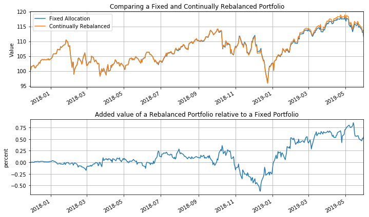
plt.figure(figsize=(10,6))

plt.subplot(2,1,1)
W_fixed.plot()
W_rebal.plot()
plt.legend(['Fixed Allocation','Continually Rebalanced'])
plt.ylabel('Value')
plt.title('Comparing a Fixed and Continually Rebalanced Portfolio')
plt.grid(True)

plt.subplot(2,1,2)
(100.0*(W_rebal-W_fixed)/W_fixed).plot()
plt.title('Added value of a Rebalanced Portfolio relative to a Fixed Portfolio')
plt.ylabel('percent')
plt.grid(True)

plt.tight_layout()

8.5.6.2. Component returns

Given data on the prices for a set of assets over an historical period \(t_0, t_1, \ldots, t_K\), an estimate the mean arithmetic return is given by the mean value

\[\begin{split} \begin{align*} \hat{r}_{j,t_K} & = \frac{1}{K}\sum_{k=1}^{K} r_{t_k} \\ & = \sum_{k=1}^{K} \frac{S_{j,t_{k}}-S_{j,t_{k-1}}}{S_{j,t_{k-1}}} \end{align*} \end{split}\]

At any point in time, \(t_k\), a mean return can be computed using the previous \(H\) intervals

\[\begin{split} \begin{align*} \hat{r}^H_{j,t_k} & = \frac{1}{H}\sum_{h=0}^{H-1} r_{t_{k-h}} \\ & = \frac{1}{H} \sum_{h=0}^{H-1}\frac{S_{j,t_{k-h}} - S_{j,t_{k-h-1}}}{S_{j,t_{k-h-1}}} \end{align*} \end{split}\]

Arithmetic returns are computed so that subsequent calculations combine returns across components of a portfolio.

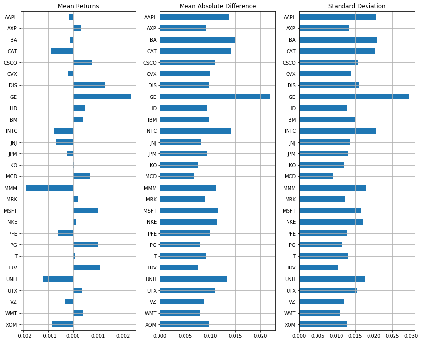
8.5.7. Measuring deviation in component returns

8.5.7.1. Mean absolute deviation

def roll(H):
    """Plot mean returns, mean absolute deviation, and standard deviation for last H days."""
    K = len(S.index)
    R = S[K-H-1:K].diff()[1:]/S[K-H-1:K].shift(1)[1:]
    AD = abs(R - R.mean())
    
    plt.figure(figsize = (12, 0.35*len(R.columns)))
    ax = [plt.subplot(1,3,i+1) for i in range(0,3)]
    
    idx = R.columns.argsort()[::-1]

    R.mean().iloc[idx].plot(ax=ax[0], kind='barh')
    ax[0].set_title('Mean Returns');
    
    AD.mean().iloc[idx].plot(ax=ax[1], kind='barh')
    ax[1].set_title('Mean Absolute Difference')

    R.std().iloc[idx].plot(ax=ax[2], kind='barh')
    ax[2].set_title('Standard Deviation')
    
    for a in ax: a.grid(True)
    plt.tight_layout()

roll(500)

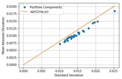
8.5.7.2. Comparing mean absolute deviation to standard deviation

R = (S.diff()[1:]/S.shift(1)[1:]).dropna(axis=0, how='all')
AD = abs(R - R.mean())

plt.plot(R.std(), AD.mean(), 'o')
plt.xlabel('Standard Deviation')
plt.ylabel('Mean Absolute Deviation')

plt.plot([0,R.std().max()],[0,np.sqrt(2.0/np.pi)*R.std().max()])
plt.legend(['Portfolio Components','sqrt(2/np.pi)'],loc='best')
plt.grid(True)

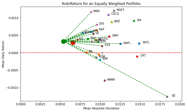
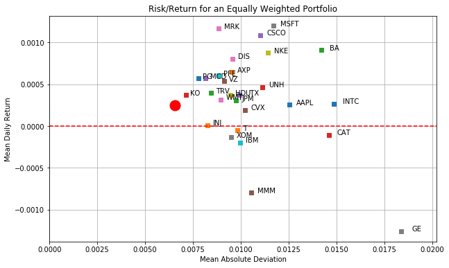
8.5.7.3. Return versus mean absolute deviation for an equally weighted continually rebalanced portfolio

plt.figure(figsize=(10,6))
for s in portfolio:
    plt.plot(AD[s].mean(), R[s].mean(),'s')
    plt.text(AD[s].mean()*1.03, R[s].mean(), s)
    
R_equal = W_rebal.diff()[1:]/W_rebal[1:]
M_equal = abs(R_equal-R_equal.mean()).mean()

plt.plot(M_equal, R_equal.mean(), 'ro', ms=15)

plt.xlim(0, 1.1*max(AD.mean()))
plt.ylim(min(0, 1.1*min(R.mean())), 1.1*max(R.mean()))
plt.plot(plt.xlim(),[0,0],'r--');
plt.title('Risk/Return for an Equally Weighted Portfolio')
plt.xlabel('Mean Absolute Deviation')
plt.ylabel('Mean Daily Return');
plt.grid(True)

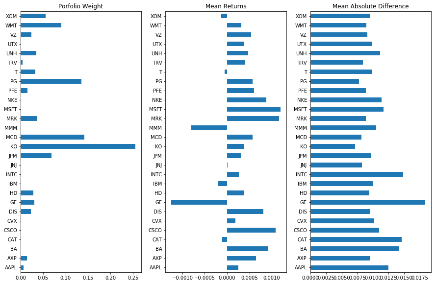
8.5.8. MAD porfolio

The linear program is formulated and solved using the pulp package.

R.head()

	AAPL	AXP	BA	CAT	CSCO	CVX	DIS	GE	HD	IBM	...	NKE	PFE	PG	T	TRV	UNH	UTX	VZ	WMT	XOM
2017-11-29	-0.020743	0.013855	0.004888	-0.006691	-0.006627	0.006269	0.017697	0.003804	0.008892	0.007083	...	0.013090	0.010041	-0.000223	0.029929	0.011428	0.031184	0.003823	0.022122	0.008164	0.007346
2017-11-30	0.013984	0.011491	0.027850	0.022382	-0.004802	0.015446	-0.003991	-0.010278	0.014500	0.002735	...	0.000995	0.001382	0.006824	-0.002742	0.007731	0.027100	0.027844	0.019841	-0.003383	0.012398
2017-12-01	-0.004655	0.001535	-0.019581	0.002621	0.008042	0.004370	0.004103	-0.022419	0.003337	0.005131	...	-0.005629	0.002482	0.004112	0.003298	0.004720	-0.006092	-0.010951	0.007073	0.001235	0.002042
2017-12-04	-0.007308	0.007460	0.024283	-0.000141	0.003191	0.011129	0.047221	0.003917	0.024831	0.010985	...	0.003674	-0.007978	0.011620	0.021096	0.001101	-0.023635	-0.000666	0.009171	-0.003493	0.001318
2017-12-05	-0.000943	0.001217	-0.008742	-0.009611	-0.010868	-0.003724	-0.027218	-0.010588	-0.011087	-0.007094	...	0.005325	-0.011926	-0.000110	-0.019318	-0.007627	-0.006007	0.002082	-0.015468	0.008453	-0.008137

5 rows × 28 columns

The decision variables will be indexed by date/time. The pandas dataframes containing the returns data are indexed by timestamps that include characters that cannot be used by the GLPK solver. Therefore we create a dictionary to translate the pandas timestamps to strings that can be read as members of a GLPK set. The strings denote seconds in the current epoch as defined by python.

a = R - R.mean()
a.head()

	AAPL	AXP	BA	CAT	CSCO	CVX	DIS	GE	HD	IBM	...	NKE	PFE	PG	T	TRV	UNH	UTX	VZ	WMT	XOM
2017-11-29	-0.020998	0.013211	0.003979	-0.006585	-0.007715	0.006077	0.016889	0.005060	0.008521	0.007281	...	0.012214	0.009439	-0.000793	0.029980	0.011030	0.030717	0.003451	0.021583	0.007846	0.007479
2017-11-30	0.013729	0.010847	0.026940	0.022488	-0.005891	0.015254	-0.004798	-0.009022	0.014129	0.002932	...	0.000119	0.000780	0.006255	-0.002692	0.007334	0.026633	0.027473	0.019302	-0.003701	0.012531
2017-12-01	-0.004910	0.000892	-0.020491	0.002727	0.006954	0.004178	0.003295	-0.021163	0.002966	0.005328	...	-0.006505	0.001880	0.003543	0.003348	0.004323	-0.006559	-0.011323	0.006534	0.000917	0.002175
2017-12-04	-0.007563	0.006817	0.023374	-0.000035	0.002103	0.010937	0.046413	0.005173	0.024461	0.011182	...	0.002798	-0.008580	0.011051	0.021147	0.000704	-0.024102	-0.001038	0.008632	-0.003811	0.001451
2017-12-05	-0.001198	0.000574	-0.009651	-0.009505	-0.011957	-0.003916	-0.028025	-0.009331	-0.011457	-0.006897	...	0.004449	-0.012528	-0.000680	-0.019268	-0.008024	-0.006474	0.001711	-0.016007	0.008135	-0.008004

5 rows × 28 columns

from pyomo.environ import *

a = R - R.mean()

m = ConcreteModel()

m.w = Var(R.columns, domain=NonNegativeReals)
m.y = Var(R.index, domain=NonNegativeReals)

m.MAD = Objective(expr=sum(m.y[t] for t in R.index)/len(R.index), sense=minimize)

m.c1 = Constraint(R.index, rule = lambda m, t: m.y[t] + sum(a.loc[t,s]*m.w[s] for s in R.columns) >= 0)
m.c2 = Constraint(R.index, rule = lambda m, t: m.y[t] - sum(a.loc[t,s]*m.w[s] for s in R.columns) >= 0)
m.c3 = Constraint(expr=sum(R[s].mean()*m.w[s] for s in R.columns) >= R_equal.mean())
m.c4 = Constraint(expr=sum(m.w[s] for s in R.columns)==1)

SolverFactory('glpk').solve(m)

w = {s: m.w[s]() for s in R.columns}

plt.figure(figsize = (15,0.35*len(R.columns)))

plt.subplot(1,3,1)
pd.Series(w).plot(kind='barh')
plt.title('Porfolio Weight');

plt.subplot(1,3,2)
R.mean().plot(kind='barh')
plt.title('Mean Returns');

plt.subplot(1,3,3)
AD.mean().plot(kind='barh')
plt.title('Mean Absolute Difference');

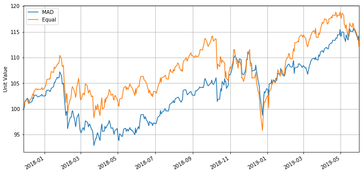
P_mad = pd.Series(0, index=S.index)
for s in portfolio:
    P_mad += 100.0*w[s]*S[s]/S[s][0]
    
plt.figure(figsize=(12,6))
P_mad.plot()
W_rebal.plot()
plt.legend(['MAD','Equal'],loc='best')
plt.ylabel('Unit Value')
plt.grid(True)

plt.figure(figsize=(10,6))
for s in portfolio:
    plt.plot(AD[s].mean(), R[s].mean(),'s')
    plt.text(AD[s].mean()*1.03, R[s].mean(), s)
    
#R_equal = P_equal.diff()[1:]/P_equal[1:]
R_equal = np.log(W_rebal/W_rebal.shift(+1))
M_equal = abs(R_equal-R_equal.mean()).mean()

plt.plot(M_equal, R_equal.mean(), 'ro', ms=15)

#R_mad = P_mad.diff()[1:]/P_mad[1:]
R_mad = np.log(P_mad/P_mad.shift(+1))
M_mad = abs(R_mad-R_mad.mean()).mean()

plt.plot(M_mad, R_mad.mean(), 'go', ms=15)

for s in portfolio:
    if w[s] >= 0.0001:
        plt.plot([M_mad, AD[s].mean()],[R_mad.mean(), R[s].mean()],'g--')
    if w[s] <= -0.0001:
        plt.plot([M_mad, AD[s].mean()],[R_mad.mean(), R[s].mean()],'r--')

plt.xlim(0, 1.1*max(AD.mean()))
plt.ylim(min(0, 1.1*min(R.mean())), 1.1*max(R.mean()))
plt.plot(plt.xlim(),[0,0],'r--');
plt.title('Risk/Return for an Equally Weighted Portfolio')
plt.xlabel('Mean Absolute Deviation')
plt.ylabel('Mean Daily Return')

Text(0, 0.5, 'Mean Daily Return')