5.8. Recharging Strategy for an Electric Vehicle#
Whether it is to visit family, take a sightseeing tour or call on business associates, planning a road trip is a familiar and routine task. Here we consider a road trip on a pre-determined route for which need to plan rest and recharging stops. This example demonstrates use of Pyomo disjunctions to model the decisions on where to stop.
# Import Pyomo and solvers for Google Colab
import sys
if "google.colab" in sys.modules:
    !wget -N -q https://raw.githubusercontent.com/jckantor/MO-book/main/tools/install_on_colab.py
    %run install_on_colab.py
installing pyomo . pyomo installed
installing and testing solvers ...
.. glpk installed
.. ipopt
.. gecode
.. couenne
.. bonmin
.. gurobi_direct installed
.. cbc installed
installation and testing complete
<Figure size 432x288 with 0 Axes>
5.8.1. Problem Statement#
The distances to the charging stations are measured relative to an arbitrary location. Given the current location \(x\), battery charge \(c\), and planning horizon \(D\), the task is to plan a series of recharging and rest stops. The objective is to drive from location \(x\) to location \(x + D\) in as little time as possible subject to the following constraints:
To allow for unforeseen events, the state of charge should never drop below 20% of the maximum capacity.
The the maximum charge is \(c_{max} = 80\) kwh.
For comfort, no more than 4 hours should pass between stops, and that a rest stop should last at least \(t^{rest}\).
Any stop includes a \(t^{lost} = 10\) minutes of “lost time”.
For this first model we make several simplifying assumptions that can be relaxed as a later time.
Travel is at a constant speed \(v = 100\) km per hour and a constant discharge rate \(R = 0.24\) kwh/km
The batteries recharge at a constant rate determined by the charging station.
Only consider stops at the recharging stations.
5.8.2. Charging Station Information#
import numpy as np
import matplotlib.pyplot as plt
import pandas as pd

# specify number of charging stations
n_charging_stations = 20

# randomly distribute charging stations along a fixed route
np.random.seed(1842)
d = np.round(np.cumsum(np.random.triangular(20, 150, 223, n_charging_stations)), 1)

# randomly assign changing capacities
c = np.random.choice([50, 100, 150, 250], n_charging_stations, p=[0.2, 0.4, 0.3, 0.1])

# assign names to the charging stations
s = [f"S_{i:02d}" for i in range(n_charging_stations)]

stations = pd.DataFrame([s, d, c]).T
stations.columns=["name", "location", "kw"]
display(stations)
| name | location | kw | |
|---|---|---|---|
| 0 | S_00 | 191.6 | 150 |
| 1 | S_01 | 310.6 | 100 |
| 2 | S_02 | 516.0 | 50 |
| 3 | S_03 | 683.6 | 50 |
| 4 | S_04 | 769.9 | 50 |
| 5 | S_05 | 869.7 | 100 |
| 6 | S_06 | 1009.1 | 150 |
| 7 | S_07 | 1164.7 | 100 |
| 8 | S_08 | 1230.8 | 100 |
| 9 | S_09 | 1350.8 | 250 |
| 10 | S_10 | 1508.4 | 100 |
| 11 | S_11 | 1639.8 | 100 |
| 12 | S_12 | 1809.4 | 150 |
| 13 | S_13 | 1947.3 | 250 |
| 14 | S_14 | 2145.2 | 150 |
| 15 | S_15 | 2337.5 | 100 |
| 16 | S_16 | 2415.6 | 100 |
| 17 | S_17 | 2590.0 | 100 |
| 18 | S_18 | 2691.2 | 100 |
| 19 | S_19 | 2896.2 | 100 |
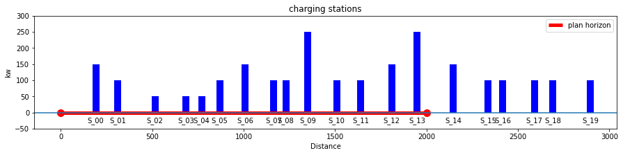
5.8.3. Route Information#
# current location (km) and charge (kw)
x = 0

# planning horizon
D = 2000

# visualize
fig, ax = plt.subplots(1, 1, figsize=(15, 3))

def plot_stations(stations, x, D, ax=ax):

    for station in stations.index:
        xs = stations.loc[station, "location"]
        ys = stations.loc[station, "kw"]
        ax.plot([xs, xs], [0, ys], 'b', lw=10, solid_capstyle="butt")
        ax.text(xs, 0-30, stations.loc[station, "name"], ha="center")

    ax.plot([x, x+D], [0, 0], 'r', lw=5, solid_capstyle="butt", label="plan horizon")
    ax.plot([x, x+D], [0, 0], 'r.', ms=20)

    ax.axhline(0)
    ax.set_ylim(-50, 300)
    ax.set_xlabel('Distance')
    ax.set_ylabel('kw')
    ax.set_title("charging stations")
    ax.legend()

plot_stations(stations, x, D)
5.8.4. Car Information#
# charge limits (kw)
c_max = 120
c_min = 0.2 * c_max
c = c_max

# velocity km/hr and discharge rate kwh/km
v = 100.0

# discharge rate in kwh/km
R = 0.24

# lost time at each stop
t_lost = 10/60
5.8.5. Model Development#
on_route = stations[(stations["location"] >= x) & (stations["location"] <= x + D)]
5.8.6. Modeling#
The problem statement identifies four state variables.
\(c\) the current battery charge
\(t\) elapsed time since the start of the trip
\(x\) the current location
The charging stations are located at positions \(d_i\) for \(i\in I\) with capacity \(C_i\). The arrival time at charging station \(i\) is given by
where the script \(t_{i-1}^{dep}\) refers to departure from the prior location. At each charging location there is a decision to make of whether to stop, rest, and rechange. If the decision is positive, then
which account for the battery charge, the lost time and time required for battery charging, and allows for a minimum rest time. On the other hand, if a decision is make to skip the charging and rest opportunity,
The latter sets of constraints have an exclusive-or relationship. That is, either one or the other of the constraint sets hold, but not both.
5.8.7. Pyomo Model#
5.8.8. Model Development#
import pyomo.environ as pyo
import pyomo.gdp as gdp

def ev_plan(stations, x, D):

    # find stations between x and x + D
    on_route = stations[(stations["location"] >= x) & (stations["location"] <= x + D)]

    m = pyo.ConcreteModel()

    m.n = pyo.Param(default=len(on_route))

    # locations and road segments between location x and x + D
    m.STATIONS = pyo.RangeSet(1, m.n)
    m.LOCATIONS = pyo.RangeSet(0, m.n + 1)
    m.SEGMENTS = pyo.RangeSet(1, m.n + 1)

    # distance traveled
    m.x = pyo.Var(m.LOCATIONS, domain=pyo.NonNegativeReals, bounds=(0, 10000))

    # arrival and departure charge at each charging station
    m.c_arr = pyo.Var(m.LOCATIONS, domain=pyo.NonNegativeReals, bounds=(c_min, c_max))
    m.c_dep = pyo.Var(m.LOCATIONS, domain=pyo.NonNegativeReals, bounds=(c_min, c_max))

    # arrival and departure times from each charging station
    m.t_arr = pyo.Var(m.LOCATIONS, domain=pyo.NonNegativeReals, bounds=(0, 100))
    m.t_dep = pyo.Var(m.LOCATIONS, domain=pyo.NonNegativeReals, bounds=(0, 100))

    # initial conditions
    m.x[0].fix(x)
    m.t_dep[0].fix(0.0)
    m.c_dep[0].fix(c)

    @m.Param(m.STATIONS)
    def C(m, i):
        return on_route.loc[i-1, "kw"]

    @m.Param(m.LOCATIONS)
    def location(m, i):
        if i == 0:
            return x
        elif i == m.n + 1:
            return x + D
        else:
            return on_route.loc[i-1, "location"]

    @m.Param(m.SEGMENTS)
    def dist(m, i):
        return m.location[i] - m.location[i-1]

    @m.Objective(sense=pyo.minimize)
    def min_time(m):
        return m.t_arr[m.n + 1]

    @m.Constraint(m.SEGMENTS)
    def drive_time(m, i):
        return m.t_arr[i] == m.t_dep[i-1] + m.dist[i]/v

    @m.Constraint(m.SEGMENTS)
    def drive_distance(m, i):
        return m.x[i] == m.x[i-1] + m.dist[i]

    @m.Constraint(m.SEGMENTS)
    def discharge(m, i):
        return m.c_arr[i] == m.c_dep[i-1] - R*m.dist[i]

    @m.Disjunction(m.STATIONS, xor=True)
    def recharge(m, i):
        # list of constraints thtat apply if there is no stop at station i
        disjunct_1 = [m.c_dep[i] == m.c_arr[i],
                      m.t_dep[i] == m.t_arr[i]]

        # list of constraints that apply if there is a stop at station i
        disjunct_2 = [m.t_dep[i] == t_lost + m.t_arr[i] + (m.c_dep[i] - m.c_arr[i])/m.C[i],
                      m.c_dep[i] >= m.c_arr[i]]

        # return a list disjuncts
        return [disjunct_1, disjunct_2]

    pyo.TransformationFactory("gdp.bigm").apply_to(m)
    pyo.SolverFactory('cbc').solve(m)

    return m

m = ev_plan(stations, 0, 1000)

results = pd.DataFrame({
    i : {"location": m.x[i](),
         "t_arr": m.t_arr[i](),
         "t_dep": m.t_dep[i](),
         "c_arr": m.c_arr[i](),
         "c_dep": m.c_dep[i](),
        } for i in m.LOCATIONS
}).T

results["t_stop"] = results["t_dep"] - results["t_arr"]

display(results)
| location | t_arr | t_dep | c_arr | c_dep | t_stop | |
|---|---|---|---|---|---|---|
| 0 | 0.0 | NaN | 0.000000 | NaN | 120.000 | NaN |
| 1 | 191.6 | 1.916000 | 1.916000 | 74.016 | 74.016 | 0.000000 |
| 2 | 310.6 | 3.106000 | 4.018107 | 45.456 | 120.000 | 0.912107 |
| 3 | 516.0 | 6.072107 | 6.072107 | 70.704 | 70.704 | 0.000000 |
| 4 | 683.6 | 7.748107 | 8.678453 | 30.480 | 68.664 | 0.930347 |
| 5 | 769.9 | 9.541453 | 9.541453 | 47.952 | 47.952 | 0.000000 |
| 6 | 869.7 | 10.539453 | 11.018840 | 24.000 | 55.272 | 0.479387 |
| 7 | 1000.0 | 12.321840 | NaN | 24.000 | NaN | NaN |
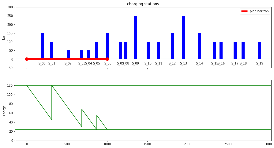
# visualize

def visualize(m, D):

    results = pd.DataFrame({
        i : {"location": m.x[i](),
             "t_arr": m.t_arr[i](),
             "t_dep": m.t_dep[i](),
             "c_arr": m.c_arr[i](),
             "c_dep": m.c_dep[i](),
            } for i in m.LOCATIONS
    }).T

    fig, ax = plt.subplots(2, 1, figsize=(15, 8), sharex=True)

    for station in stations.index:
        xs = stations.loc[station, "location"]
        ys = stations.loc[station, "kw"]
        ax[0].plot([xs, xs], [0, ys], 'b', lw=10, solid_capstyle="butt")
        ax[0].text(xs, 0-30, stations.loc[station, "name"], ha="center")

    ax[0].plot([x, x+D], [0, 0], 'r', lw=5, solid_capstyle="butt", label="plan horizon")
    ax[0].plot([x, x+D], [0, 0], 'r.', ms=20)

    ax[0].axhline(0)
    ax[0].set_ylim(-50, 300)
    ax[0].set_ylabel('kw')
    ax[0].set_title("charging stations")
    ax[0].legend()

    for i in m.SEGMENTS:
        xv = [results.loc[i-1, "location"], results.loc[i, "location"]]
        cv = [results.loc[i-1, "c_dep"], results.loc[i, "c_arr"]]
        ax[1].plot(xv, cv, 'g')

    for i in m.STATIONS:
        xv = [results.loc[i, "location"]]*2
        cv = [results.loc[i, "c_arr"], results.loc[i, "c_dep"]]
        ax[1].plot(xv, cv, 'g')

    ax[1].axhline(c_max, c='g')
    ax[1].axhline(c_min, c='g')
    ax[1].set_ylim(0, 1.1*c_max)
    ax[1].set_ylabel('Charge')

visualize(ev_plan(stations, 0, 1000), 1000)
5.8.9. Suggested Exercises#
Does increasing the battery capacity \(c^{max}\) significantly reduce the time required to travel 2000 km? Explain what you observe.
“The best-laid schemes of mice and men go oft awry” (Robert Burns, “To a Mouse”). Modify this model so that it can be used to update a plans in response to real-time measurements. How does the charging strategy change as a function of planning horizon \(D\)?