5.2. Linear Blending Problems#
This notebook introduces material blending problems and outlines a multi-step procedure for developing and solving models using Pyomo.
5.2.1. Learning Goals#
Linear Blending problems
Frequently encountered in material blending
Models generally consist of linear mixing rules and mass/material balances
Decision variables are indexed by a set of raw materials
Further practice with key elements of modeling for optimization
pyo.ConcreteModel()to create a new instancce of an optimization modelpyo.Set()to create an index used to index decision variablespyo.Var()to create an optimization decision variablemodel.Comstraint()to decorate (tag) the output of a function as an optimization constraintmodel.Objective()to decorate (tag) the output of a function as an optimization objective
Modeling and solving linear blending problems in CVXPY
Step 1. Coding problem data. Nested dictionaries or Pandas dataframes.
Step 2. Create index set. Use .keys() with nested dictionaries, or .index with Pandas dataframes.
Step 3. Create a dictionary of decision variables. Add any pertinent qualifiers or constraints for individual variables such as lower and upper bounds, non-negativity, variable names.
Step 4. Create an expression defining the problem objective.
Step 5. Create a one or more lists of problem constraints.
Step 6. Create the problem object from the objectives and constraints.
Step 7. Solve and display the solution.
5.2.2. Problem Statement (Jenchura, 2017)#
A brewery receives an order for 100 gallons that is at least 4% ABV (alchohol by volume) beer. The brewery has on hand beer A that is 4.5% ABV and costs \\(0.32 per gallon to make, and beer B that is 3.7% ABV and costs \\\)0.25 per gallon. Water (W) can also be used as a blending agent at a cost of \$0.05 per gallon. Find the minimum cost blend of A, B, and W that meets the customer requirements.
5.2.3. Analysis#
Before going futher, carefully read the problem description with the following questions in mind.
What are the decision variables?
What is the objective?
What are the constraints?
5.2.3.1. Decision variables#
The decision variables for this problem are the amounts of blending stocks “A”, “B”, and “W” to included in the final batch. We can define a set of blending stocks \(S\), and non-negative decision variables \(x_s\) that are indexed by the components in \(S\) that denote the amount of \(s\) included in the final batch.
5.2.3.2. Objective#
If we designate the price of blending stock \(s \in S\) as \(P_s\), the cost is
The objective is to minimize cost.
5.2.3.3. Constraints#
5.2.3.3.1. Order Volume#
Let \(V = 100\) represent the desired volume of product and assume ideal mixing. Then
5.2.3.3.2. Alcohol by Volume#
Let \(C_s\) denote the volume fraction of alcohol in blending stock \(s\). Assuming ideal mixing, the total volume of of alchohol in the final product be
If \(\bar{C}\) denotes the required average concentration, then
Which is not linear in the decision variables. If at all possible, linear constraints are much preferred because (1) they enable the use of LP solvers, and (2) then tend to avoid problems that can arise with division by zero and other issues.
There are other ways to write composition constraints, but this one is preferred because it isolates the product quality parameter, \(\bar{C}\), in a single constraint. This constraint has “one job to do”.
5.2.4. Solving optimization problems with Pyomo#
5.2.4.1. Step 1. Coding Problem Data as a Pandas DataFrame#
The first step is to represent the problem data in a generic manner that could be extended to include additional blending components. Here we use a Pandas dataframe of raw materials, each row representing a unique blending agent, and columns containing attributes of the blending components. This is consistent with “Tidy Data” principles.
data = pd.DataFrame([
    ['A', 0.045, 0.32],
    ['B', 0.037, 0.25],
    ['W', 0.000, 0.05]],
    columns = ['blending stock', 'Concentration', 'Price']
)

data.set_index('blending stock', inplace=True)
display(data)
| Concentration | Price | |
|---|---|---|
| blending stock | ||
| A | 0.045 | 0.32 |
| B | 0.037 | 0.25 |
| W | 0.000 | 0.05 |
5.2.4.2. Step 2. Creating a model instance#
import numpy as np
import pyomo.environ as pyo
import pandas as pd

bm = pyo.ConcreteModel('Blending Model')
5.2.4.3. Step 3. Identifying index sets#
The objectives and constraints encountered in optimization problems often include sums over a set of objects. In the case, we will need to create sums over the set of blending stocks. We will use these index sets to create decision variables and to express the sums that appear in the objective and constraints
data.index
Index(['A', 'B', 'W'], dtype='object', name='blending stock')
bm.S = pyo.Set(initialize=data.index)

for s in bm.S:
    print(s)
A
B
W
5.2.4.4. Step 4. Create decision variables#
Most real-world applications of optimization technologies involve many decision variables and constraints. It would be impractical to create unique identifiers for literally thousands of variables. For this reason, the pyo.Var() and other objects can create indexed sets of variables and constraints. Here is how it is done for the blending problem.
bm.x = pyo.Var(bm.S, domain=pyo.NonNegativeReals)
5.2.4.5. Step 4. Objective Function#
If we let subscript \(d\) denote a blending d from the set of blending components \(C\), and denote the volume of \(c\) used in the blend as \(x_c\), the cost of the blend is
where \(P_s\) is the price per unit volume of \(s\). Using the Python data dictionary defined above, the price \(P_s\) is given by data[s, 'Price']
@bm.Objective(sense=pyo.minimize)
def cost(bm):
    return sum(bm.x[s] * data.loc[s, "Price"] for s in bm.S)

bm.cost.pprint()
WARNING: Implicitly replacing the Component attribute cost (type=<class
    'pyomo.core.base.objective.ScalarObjective'>) on block Blending Model with
    a new Component (type=<class
    'pyomo.core.base.objective.ScalarObjective'>). This is usually indicative
    of a modelling error. To avoid this warning, use block.del_component() and
    block.add_component().
cost : Size=1, Index=None, Active=True
    Key  : Active : Sense    : Expression
    None :   True : minimize : 0.32*x[A] + 0.25*x[B] + 0.05*x[W]
5.2.4.6. Step 5. Constraints#
5.2.4.6.1. Volume Constraint#
The customer requirement is produce a total volume \(V\). Assuming ideal solutions, the constraint is given by
where \(x_s\) denotes the volume of blending stock \(s\) used in the blend.
V = 100

@bm.Constraint()
def volume(bm):
    return sum(bm.x[s] for s in bm.S) == V

bm.volume.pprint()
WARNING: Implicitly replacing the Component attribute volume (type=<class
    'pyomo.core.base.constraint.ScalarConstraint'>) on block Blending Model
    with a new Component (type=<class
    'pyomo.core.base.constraint.AbstractScalarConstraint'>). This is usually
    indicative of a modelling error. To avoid this warning, use
    block.del_component() and block.add_component().
volume : Size=1, Index=None, Active=True
    Key  : Lower : Body               : Upper : Active
    None : 100.0 : x[A] + x[B] + x[W] : 100.0 :   True
5.2.4.6.2. Composition Constraint#
C_lb = 0.04

@bm.Constraint()
def composition(bm):
    return sum(bm.x[s]*(data.loc[s, "Concentration"] - C_lb) for s in bm.S) >= 0

bm.composition.pprint()
WARNING: Implicitly replacing the Component attribute composition (type=<class
    'pyomo.core.base.constraint.ScalarConstraint'>) on block Blending Model
    with a new Component (type=<class
    'pyomo.core.base.constraint.AbstractScalarConstraint'>). This is usually
    indicative of a modelling error. To avoid this warning, use
    block.del_component() and block.add_component().
composition : Size=1, Index=None, Active=True
    Key  : Lower : Body                                                                : Upper : Active
    None :   0.0 : 0.0049999999999999975*x[A] - 0.0030000000000000027*x[B] - 0.04*x[W] :  +Inf :   True
5.2.4.7. Step 6. Solve#
bm.pprint()
1 Set Declarations
    S : Size=1, Index=None, Ordered=Insertion
        Key  : Dimen : Domain : Size : Members
        None :     1 :    Any :    3 : {'A', 'B', 'W'}

1 Var Declarations
    x : Size=3, Index=S
        Key : Lower : Value : Upper : Fixed : Stale : Domain
          A :     0 :  None :  None : False :  True : NonNegativeReals
          B :     0 :  None :  None : False :  True : NonNegativeReals
          W :     0 :  None :  None : False :  True : NonNegativeReals

1 Objective Declarations
    cost : Size=1, Index=None, Active=True
        Key  : Active : Sense    : Expression
        None :   True : minimize : 0.32*x[A] + 0.25*x[B] + 0.05*x[W]

2 Constraint Declarations
    composition : Size=1, Index=None, Active=True
        Key  : Lower : Body                                                                : Upper : Active
        None :   0.0 : 0.0049999999999999975*x[A] - 0.0030000000000000027*x[B] - 0.04*x[W] :  +Inf :   True
    volume : Size=1, Index=None, Active=True
        Key  : Lower : Body               : Upper : Active
        None : 100.0 : x[A] + x[B] + x[W] : 100.0 :   True

5 Declarations: S x cost volume composition
solver = pyo.SolverFactory('glpk')
solver.solve(bm, tee=True).write()
GLPSOL--GLPK LP/MIP Solver 5.0
Parameter(s) specified in the command line:
 --write /var/folders/cm/z3t28j296f98jdp1vqyplkz00000gn/T/tmpr_905u1e.glpk.raw
 --wglp /var/folders/cm/z3t28j296f98jdp1vqyplkz00000gn/T/tmpkqr7abph.glpk.glp
 --cpxlp /var/folders/cm/z3t28j296f98jdp1vqyplkz00000gn/T/tmp4_k2zpfj.pyomo.lp
Reading problem data from '/var/folders/cm/z3t28j296f98jdp1vqyplkz00000gn/T/tmp4_k2zpfj.pyomo.lp'...
3 rows, 4 columns, 7 non-zeros
30 lines were read
Writing problem data to '/var/folders/cm/z3t28j296f98jdp1vqyplkz00000gn/T/tmpkqr7abph.glpk.glp'...
23 lines were written
GLPK Simplex Optimizer 5.0
3 rows, 4 columns, 7 non-zeros
Preprocessing...
2 rows, 3 columns, 6 non-zeros
Scaling...
 A: min|aij| =  3.000e-03  max|aij| =  1.000e+00  ratio =  3.333e+02
GM: min|aij| =  5.233e-01  max|aij| =  1.911e+00  ratio =  3.651e+00
EQ: min|aij| =  2.739e-01  max|aij| =  1.000e+00  ratio =  3.651e+00
Constructing initial basis...
Size of triangular part is 2
      0: obj =   5.000000000e+00 inf =   1.911e+02 (1)
      1: obj =   2.900000000e+01 inf =   0.000e+00 (0)
*     2: obj =   2.762500000e+01 inf =   0.000e+00 (0)
OPTIMAL LP SOLUTION FOUND
Time used:   0.0 secs
Memory used: 0.0 Mb (40412 bytes)
Writing basic solution to '/var/folders/cm/z3t28j296f98jdp1vqyplkz00000gn/T/tmpr_905u1e.glpk.raw'...
16 lines were written
# ==========================================================
# = Solver Results                                         =
# ==========================================================
# ----------------------------------------------------------
#   Problem Information
# ----------------------------------------------------------
Problem:
- Name: unknown
  Lower bound: 27.625
  Upper bound: 27.625
  Number of objectives: 1
  Number of constraints: 3
  Number of variables: 4
  Number of nonzeros: 7
  Sense: minimize
# ----------------------------------------------------------
#   Solver Information
# ----------------------------------------------------------
Solver:
- Status: ok
  Termination condition: optimal
  Statistics:
    Branch and bound:
      Number of bounded subproblems: 0
      Number of created subproblems: 0
  Error rc: 0
  Time: 0.013801097869873047
# ----------------------------------------------------------
#   Solution Information
# ----------------------------------------------------------
Solution:
- number of solutions: 0
  number of solutions displayed: 0
5.2.4.8. Step 7. Display solution#
Following solution, the values of any Pyomo variable, expression, objective, or constraint can be accessed using the associated value property.
bm.pprint()
1 Set Declarations
    S : Size=1, Index=None, Ordered=Insertion
        Key  : Dimen : Domain : Size : Members
        None :     1 :    Any :    3 : {'A', 'B', 'W'}

1 Var Declarations
    x : Size=3, Index=S
        Key : Lower : Value            : Upper : Fixed : Stale : Domain
          A :     0 : 37.5000000000001 :  None : False : False : NonNegativeReals
          B :     0 :             62.5 :  None : False : False : NonNegativeReals
          W :     0 :              0.0 :  None : False : False : NonNegativeReals

1 Objective Declarations
    cost : Size=1, Index=None, Active=True
        Key  : Active : Sense    : Expression
        None :   True : minimize : 0.32*x[A] + 0.25*x[B] + 0.05*x[W]

2 Constraint Declarations
    composition : Size=1, Index=None, Active=True
        Key  : Lower : Body                                                                : Upper : Active
        None :   0.0 : 0.0049999999999999975*x[A] - 0.0030000000000000027*x[B] - 0.04*x[W] :  +Inf :   True
    volume : Size=1, Index=None, Active=True
        Key  : Lower : Body               : Upper : Active
        None : 100.0 : x[A] + x[B] + x[W] : 100.0 :   True

5 Declarations: S x cost volume composition
print(bm.cost())
27.625000000000032
print(f"Minimum cost to produce {V} gallons at greater than ABV={C_lb}: ${bm.cost():5.2f}")
Minimum cost to produce 100 gallons at greater than ABV=0.04: $27.63
for s in bm.S:
    print(f"{s}: {bm.x[s]():6.2f} gallons")
A:  37.50 gallons
B:  62.50 gallons
W:   0.00 gallons
5.2.5. Parametric Studies#
An important use of optimization models is to investigate how operations depend on critical parameters. For example, for this blending problem we may be interested in questions like:
How does the operating cost change with product alcohol content?
What is the cost of producing one more gallon of product?
What if the supply of a raw material is constrained?
What if we produce two products rather than one?
How much would be pay for raw materials with different specifications
5.2.5.1. Consolidating the model into a single function to create and solve for optimal blend#
To enable parametric studies, our first step is to consolidate the model into a function that accepts problem data and reports an optimal solution.
import numpy as np
import pyomo.environ as pyo
import pandas as pd


def blend_beer(data, V=100, C_lb=0.04):

    # create model
    bm = pyo.ConcreteModel('Blending Model')

    # create index set for decision variables
    bm.S = pyo.Set(initialize=data.index)

    # create decision variables
    bm.x = pyo.Var(bm.S, domain=pyo.NonNegativeReals)

    # specify objective
    @bm.Objective(sense=pyo.minimize)
    def cost(bm):
        return sum(bm.x[s] * data.loc[s, "Price"] for s in bm.S)

    # volume constraint
    @bm.Constraint()
    def volume(bm):
        return sum(bm.x[s] for s in bm.S) == V

    # composition constraint
    @bm.Constraint()
    def composition(bm):
        return sum(bm.x[s]*(data.loc[s, "Concentration"] - C_lb) for s in bm.S) >= 0

    # solve model
    solver = pyo.SolverFactory('glpk')
    solver.solve(bm)

    # return model for post-processing and display
    return bm
5.2.5.2. How to use the optimization model#
# specify blending stock data
data = pd.DataFrame([
['A', 0.045, 0.32],
['B', 0.037, 0.25], ['C', .042, .28],
['W', 0.000, 0.05]],
columns = ['blending stock', 'Concentration', 'Price']
)
data.set_index('blending stock', inplace=True)
display(data)
# set product requirements
volume = 100
abv = 0.04
# compute optimal solution using optimization model
bm = blend_beer(data, volume, abv)
# extract data from the model
optimal_blend = pd.DataFrame()
optimal_blend.index = [s for s in bm.S]
optimal_blend["amount"] = [bm.x[s]() for s in bm.S]
min_cost = bm.cost()
# display solutoin
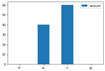
print(f"Minimum cost to produce {volume} gallons at ABV={abv} = ${min_cost:5.2f}")
display(optimal_blend)
optimal_blend.plot(y="amount", kind="bar")
| Concentration | Price | |
|---|---|---|
| blending stock | ||
| A | 0.045 | 0.32 |
| B | 0.037 | 0.25 |
| C | 0.042 | 0.28 |
| W | 0.000 | 0.05 |
Minimum cost to produce 100 gallons at ABV=0.04 = $26.80
| amount | |
|---|---|
| A | 0.0 |
| B | 40.0 |
| C | 60.0 |
| W | 0.0 |
<AxesSubplot:>
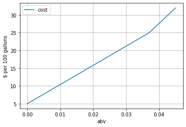
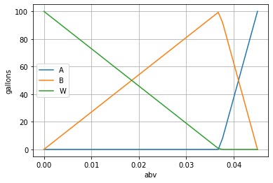
5.2.6. Parametric Study#
The following cell uses the optimal blending model to compute the minimum cost and blending stocks to produce
print(data)
volume = 100

# gather results for a range of abv values
abv = np.linspace(0, 0.045)

results = pd.DataFrame(columns=["abv", "cost", "A", "B", "W"])
for row, a in enumerate(abv):
    bm = blend_beer(data, volume, a)
    results.loc[row] = [a, bm.cost(), bm.x["A"](), bm.x["B"](), bm.x["W"]()]

results.plot(x="abv", y="cost", ylabel="$ per 100 gallons", grid=True)
results.plot(x="abv", y=["A", "B", "W"], ylabel="gallons", grid=True)
                Concentration  Price
blending stock
A                       0.045   0.32
B                       0.037   0.25
W                       0.000   0.05
<AxesSubplot:xlabel='abv', ylabel='gallons'>
5.2.7. Study Exercises#
5.2.7.1. Exercise 1#
An additional raw blending stock “C” becomes available with an abv of 4.2% at a cost of 28 cents per gallon. How does that change the optimal blend for a product volume of 100 gallons and an abv of 4.0%?
5.2.7.2. Exercise 2#
Having decided to use “C” for the blended product, you later learn only 50 gallons of “C” are available. Modify the solution procedure to allow for limits on the amount of raw maaterial, and investigate the implications for the optimal blend of having only 50 gallons of “C” available, and assuming the amounts of the other components “A”, “B”, and “W” remain unlimited.
5.2.7.3. Exercise 3#
An opportunity has developed to sell a second product with an abv of 3.8%. The first product is now labeled “X” with abv 4.0% and sells for \\(1.25 per gallon, and the second product is designated "Y" and sells for \\\)1.10 per gallon. You’ve also learned that all of your raw materials are limited to 50 gallons. What should your production plan be to maximize profits?