2.2. Lab Assignment 1: Step Test of a First-Order System

This notebook outlines a process for fitting a first-order model of a heater/sensor assembly to data taken during a step test. The learning goals for this notebook are:

• Read and plot a previously saved step test data using the Pandas library.

• By inspection, identify the gain and dominant time constant of the step test.

• Simulate the response of a first-order model to step test.

• Through iteration, adjust model parameters to fit the first order model to step test data.

• Understand the relationship of model parameters to gain and time constant.

• Determine if a first-order model provides an adequate description of the observed response.

2.2.1. Background and Starter Code

2.2.1.1. First-order lumped model for heater/sensor device.

We have previously developed a first-order model for one heater/sensor pair on the temperature control lab device. An energy balance gives

(2.1)\[\begin{align} C_p\frac{dT_1}{dt} & = U_a(T_{amb} - T_1) + \alpha P_1u_1 \\ \end{align}\]

where \(T_1\) is the average temperature of heater/sensor one, \(T_{amb}\) is the ambient temperature of the surroundings. The unknown parameters are the heat capacity \(C_p\) and the heat transfer coefficient \(U_a\).

The parameters describing the heat input are as follows:

• \(\alpha\) is a system calibration constant The measured value of \(\alpha\) is 0.16 milliwatts per unit of \(P_1\) per percent.

• \(P_1\) is a constant integer value in the range 0 to 255 that controls the operating range of heater 1. It is set using the tclab library.

• \(u_1\) is a floating point value in the range 0 to 100 that specify the percentage of available power for heater 1.

For example, if \(P_1 = 255\) and \(u_1 = 100\), then the total applied power is

\[\alpha_1 P_1 u_1 = 0.16 \times 200 \times 50 = 4080\ \text{milliwatts} = 4.08\ \text{watts}\]

2.2.1.2. Reading previously saved experimental data

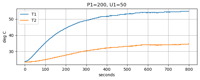
A step test was performed where the temperature control laboratory was initially at steady state at ambient temperature. The heater range \(P_1\) was set to 200, then heater 1 was set to 50% of full range with \(\bar{u}_1 = 50\). Temperatures \(T_1\) and \(T_2\) were recorded for 800 seconds. The has been saved to the course Github repository where it can be located with the url

https://raw.githubusercontent.com/jckantor/CBE30338-book/main/tclab/data/tclab-data.csv

The following cell reads the step test data using the Pandas library. The data is stored in a Pandas DataFrame called data.

import pandas as pd

# parameter values
P1 = 200
U1 = 50

# file location
github_repo = "https://raw.githubusercontent.com/jckantor/CBE30338-book/main/"
file_path = "tclab/data/tclab-data.csv"
url = github_repo + file_path

# read file
data = pd.read_csv(url, index_col="Time")

# display the step test data
display(data)

	T1	T2	Q1	Q2
Time
0.00	23.81	23.48	50.0	0.0
1.00	23.81	23.48	50.0	0.0
2.00	23.81	23.48	50.0	0.0
3.00	23.81	23.48	50.0	0.0
4.01	23.81	23.48	50.0	0.0
...	...	...	...	...
796.00	54.75	34.44	50.0	0.0
797.00	54.75	34.44	50.0	0.0
798.01	54.75	34.76	50.0	0.0
799.00	54.75	34.76	50.0	0.0
800.00	54.75	34.76	50.0	0.0

800 rows × 4 columns

Next we plot the data using the .plot() method associated with every Pandas DataFrame. The Pandas plot method provides a concise and intuitive means of plotting data.

data.plot(y=["T1", "T2"], 
          title=f"{P1=}, {U1=}",
          xlabel="seconds", 
          ylabel="deg C", 
          grid=True, 
          figsize=(8, 2.5)
         )

data.plot(y=["Q1", "Q2"],
          title=f"{P1=}, {U1=}",
          xlabel="seconds", 
          ylabel="% of full range", 
          grid=True, 
          figsize=(8, 1.5),
          ylim=(0, 100)
         )

<AxesSubplot: title={'center': 'P1=200, U1=50'}, xlabel='seconds', ylabel='% of full range'>

2.2.1.3. Analytical Solution for a Step Test

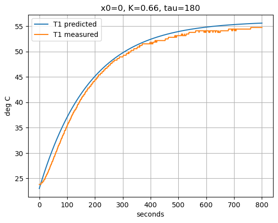
The goal of this assignment is to fit a first-order model to the step test. The strategy we use will be use an analytical solution for a first-order model subject to a step change in the input. Then, by trail-and-error, find a set of model parameters that provide a good fit to the experimental data.

We start with a first-order model written in gain/time-constant form

\[\tau\frac{dx}{dt} = -x + K \bar{u}\]

where \(x = T_1 - T_{amb}\) and the \(\bar{u}\) is a constant value for the input \(u_1(t)\). The analytical solution consists of two parts

\[x(t) = \underbrace{x_0e^{-t/\tau}}_{\text{initial condition }x_0} + \underbrace{(1 - e^{-t/\tau}) K \bar{u}}_{\text{input }\bar{u}}\]

The solution depends on three parameters:

• \(x_0\): initial condition

• \(K\): steady-state gain

• \(\tau\): time constant

The initial condition \(x_0 = 0\) if the step test starts at steady-state. In that case there are two parameters to fit, \(K\) and \(\tau\). The following cell demonstrates the calculation and plotting of the analytical solution.

import numpy as np
import matplotlib.pyplot as plt

# estimate parameter values
T_amb = 23
x0 = 0
K = 0.66
tau = 180

# known input
U1 = 50

# compute analytical solution
t = data.index
x = x0*np.exp(-t/tau) + (1 - np.exp(-t/tau))*K*U1

# plotting solution for T1
T1 = x + T_amb
plt.plot(t, T1, t, data["T1"])
plt.legend(["T1 predicted", "T1 measured"])

# dress up the plot
plt.title(f"{x0=}, {K=}, {tau=}")
plt.xlabel("seconds")
plt.ylabel("deg C")
plt.grid(True)

2.2.2. Lab Assignment

The lab assignment is to conduct a step test of the Temperature Control Lab, and then to fit the results to a first order model of a heater/sensor assembly.

Task 1.

Create a new Jupyter notebook to document the results of your step test and model fitting experiment.

• Begin the notebook with an appropriate title, description, and any information that would be required to reproduce the experiment.

• Create a cell to read the data you saved from your step test experiment. Plot the data as outlined above.

• Inspecting the plot for \(T_1\), estimate the

  • gain,

  • time constant

  • ambient temperature

Write your estimates in a clearly labeled markdown cell.

Task 2.

Following the starter code presented above, create a new cell to plot an analytical solution for the step response of a first-order model in gain/time constant form. Use your estimates of gain, time constant, initial condition, and the input. On the same plot, overlay a plot of the experimental data. Adjust parameter values until you get the a good fit of the model to the experimental data.

Note that you may need to also adjust values of the ambient temperature and initial condition to fit the model.

Report

• gain

• time constant

• ambient temperature

• initial condition

Task 3.

A first-order model in gain/time constant form is given by

\[\tau\frac{dx}{dt} = - x + K u \]

Where \(x\) is the state variable. Again letting \(x = T_1 - T_{amb}\) and \(u = u_1\) Comparing this model of a first order system to the model given up for the heater/sensor assembly.

• Derive expressions for the parameters \(\tau\) and \(K\) in terms of \(C_p\), \(U_a\), \(\alpha\), and \(P_1\).

• Assume \(\alpha = 0.16\) milliwatts per unit of \(P1\) per percent. Solve for estimates of \(C_p\) and \(U_a\).

Task 4.

In a new markdown cell, discuss issues you would face in writing a Python function to automatically fit the model of the heater/sensor assembly to step test data. Your discussion should include the following considerations:

• How can you measure the quality of fit?

• How should one handle bad measurements?

• What parameters should be fit?

• How can you estimate uncertainty in the estimates of \(C_p\) and \(U_a\)?

• Is it possible to estimate \(U_a\) from a steady state experiment?

• Is is possible to estimate \(C_p\) from a steady state experiment?