6.1. Simulation and Optimal Control in Pharmacokinetics#
6.1.1. Installations and Initialization#
Pyomo and ipopt are now preinstalled on Google Colaboratory. On MacOS and Windows PC, a one-time installation of pyomo and ipopt is required. The following commands will perform the needed installation when using the Anaconda distribution of Python.
!wget -N -q "https://ampl.com/dl/open/ipopt/ipopt-linux64.zip"
!unzip -o -q ipopt-linux64
ipopt_executable = '/content/ipopt'
import matplotlib.pyplot as plt
import pyomo.environ as pyo
import pyomo.dae as dae
On MacOS and Windows PC, a one-time installation of pyomo and ipopt is required. The following commands will perform the needed installation when using the Anaconda distribution of Python.
!conda install -c conda-forge pyomo
!conda install -c conda-forge pyomo.extras
!conda install -c conda-forge ipopt
6.1.2. A Pharmacokinetics Example#
Pharmacokinetics – the study of the drugs and other substances administered to a living organism – is a rich source of examples for simulation and optimization. Here we discuss a solution to a very simple problem.
A patient is admitted to a clinic with a dangerous blood borne infection that needs to be treated with a specific antibiotic. The treatment requires a minimum therapeutic concentration of 20 mg/liter of blood, but, for safety reasons, should not exceed 40 mg/liter. The attending physician has established a target value of 25 mg/liter. The antibiotic will be administered to the patient by continuous infusion over a 72 hour period using a pump capable of delivering up to 50 mg/hour.

(photo from Pflegewiki-User Würfel, CC BY-SA 3.0)
The research literature shows dynamics of antibiotic concentration in the body behaves according to a one-compartment pharmacokinetic model
where \(V\) is compartment volume (e.g., blood is about 5 liters in an adult), and \(kC\) is the rate of elimination due to all sources, including metabolism and excretion. Based on an observed half-life in the blood of 8 hours, \(k\) has an estimated value of 0.625 liters/hour. Given this information, what administration policy would you recommend?
6.1.3. Simulation of Fixed Infusion Rate Strategy#
The first strategy we will investigate is constant infusion. At steady-state, the pharmacokinetic model becomes
The following cell simulates the patient response.
# parameters
t_final = 72     # hours
V = 5.0          # liters
k = 0.625        # liters/hour
u = 25*0.625     # mg/hour infusion rate

# create a model
model = pyo.ConcreteModel()

# define time as a continous set with bounds
model.t = dae.ContinuousSet(bounds=(0, t_final))

# define problem variable indexed by time
model.C = pyo.Var(model.t, domain=pyo.NonNegativeReals)
model.dCdt = dae.DerivativeVar(model.C, wrt=model.t)

# the differential equation is a constraint indexed by time
@model.Constraint(model.t)
def ode(model, t):
    return V*model.dCdt[t] == u - k*model.C[t]

# initial condition
model.C[0].fix(0)

# transform the model to a system of algebraic constraints
TransformationFactory('dae.finite_difference').apply_to(model, nfe=50, method='backwards')

# compute a solution using the Pyomo simulator capability
tsim, profiles = Simulator(model, package='ioppt').simulate()

# plot results
plt.plot(tsim, profiles)
plt.xlabel('time / hours')
plt.ylabel('mg/liter')
plt.title('Blood conctration for a steady infusion of ' + str(u) + ' mg/hr.');
---------------------------------------------------------------------------
ValueError                                Traceback (most recent call last)
Input In [14], in <cell line: 26>()
     23 model.C[0].fix(0)
     25 # transform the model to a system of algebraic constraints
---> 26 TransformationFactory('dae.finite_difference').apply_to(model, nfe=50, method='backwards')
     28 # compute a solution using the Pyomo simulator capability
     29 tsim, profiles = Simulator(model, package='ioppt').simulate()

File ~/opt/anaconda3/lib/python3.9/site-packages/pyomo/core/base/transformation.py:69, in Transformation.apply_to(self, model, **kwds)
     67 if not hasattr(model, '_transformation_data'):
     68     model._transformation_data = TransformationData()
---> 69 self._apply_to(model, **kwds)
     70 timer.report()

File ~/opt/anaconda3/lib/python3.9/site-packages/pyomo/dae/plugins/finitedifference.py:169, in Finite_Difference_Transformation._apply_to(self, instance, **kwds)
    153 def _apply_to(self, instance, **kwds):
    154     """
    155     Applies the transformation to a modeling instance
    156
   (...)
    166                   scheme is the backward difference method
    167     """
--> 169     config = self.CONFIG(kwds)
    171     tmpnfe = config.nfe
    172     tmpds = config.wrt

File ~/opt/anaconda3/lib/python3.9/site-packages/pyomo/common/config.py:1231, in ConfigBase.__call__(self, value, default, domain, description, doc, visibility, implicit, implicit_domain, preserve_implicit)
   1229 # ... and set the value, if appropriate
   1230 if value is not NoArgumentGiven:
-> 1231     ans.set_value(value)
   1232 return ans

File ~/opt/anaconda3/lib/python3.9/site-packages/pyomo/common/config.py:2177, in ConfigDict.set_value(self, value, skip_implicit)
   2175             _implicit.append(key)
   2176         else:
-> 2177             raise ValueError(
   2178                 "key '%s' not defined for ConfigDict '%s' and "
   2179                 "implicit (undefined) keys are not allowed" %
   2180                 (key, self.name(True)))
   2182 # If the set_value fails part-way through the new values, we
   2183 # want to restore a deterministic state.  That is, either
   2184 # set_value succeeds completely, or else nothing happens.
   2185 _old_data = self.value(False)

ValueError: key 'method' not defined for ConfigDict '' and implicit (undefined) keys are not allowed
6.1.4. Optimizing the Infusion Strategy#
The simulation results show that a constant rate of infusion results in a prolonged period, more than twelve hours, where the antibiotic concentration is below the minimum therapuetic dose of 20 mg/liter. Can we find a better strategy? In particular, can a time-varying strategy yield reduce the time needed to achieve the therapuetic level?
For this case, we consider \(u(t)\) to be a time-varying infusion rate bounded by the capabilities of the infusion pump.
Next we need to express the objective of maintaining the antibiotic concentration at or near a value \(C_{SP}\) = 25 mg/liter. For this purpose, we define the objective as minimizing the integral square error defined as
The next cell demonstrates how to formulate the model in Pyomo, and compute a solution using ipopt.
# parameters
t_final = 72     # hours
V = 5.0          # liters
k = 0.625        # liters/hour
u_max = 50       # mg/hour infusion rate
Csp = 25         # setpoint

# create a model
model = ConcreteModel()

# define time as a continous set with bounds
model.t = ContinuousSet(bounds=(0, t_final))

# define problem variable indexed by time
model.u = Var(model.t, bounds=(0, u_max))
model.C = Var(model.t, domain=NonNegativeReals)
model.dCdt = DerivativeVar(model.C, wrt=model.t)

# the differential equation is a constraint indexed by time
model.ode = Constraint(model.t, rule=lambda model, t: V*model.dCdt[t] == model.u[t] - k*model.C[t])

# initial condition
model.C[0].fix(0)

# objective
model.ise = Integral(model.t, wrt=model.t, rule=lambda model, t: (model.C[t] - Csp)**2)
model.obj = Objective(expr=model.ise, sense=minimize)

# transform the model to a system of algebraic constraints
TransformationFactory('dae.finite_difference').apply_to(model, nfe=200, method='backwards')

# simulation
SolverFactory('ipopt', executable=ipopt_executable).solve(model)

# extract solutions from the model
tsim = [t for t in model.t]
Csim = [model.C[t]() for t in model.t]
usim = [model.u[t]() for t in model.t]

# plot results
plt.figure(figsize=(8,6))
plt.subplot(2,1,1)
plt.plot(tsim, Csim)
plt.title('Blood concentration of antibiotic')
plt.xlabel('time / hours')
plt.ylabel('mg/liter')

plt.subplot(2,1,2)
plt.plot(tsim, usim)
plt.ylim((0, 1.1*u_max))
plt.title('Infusion rate')
plt.xlabel('time / hours')
plt.ylabel('mg/hour')

plt.tight_layout()
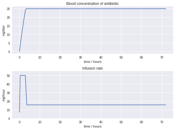
The result of this optimization is a much better therapy for the patient. Therapuetic levels of antibiotic are reach with 3 hours thereby leading to an earlier outcome and the possibility of an earlier recovery.
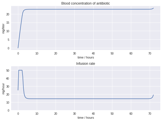
6.1.5. Alternative Objectives#
# parameters
t_final = 72     # hours
V = 5.0          # liters
k = 0.625        # liters/hour
u_max = 50       # mg/hour infusion rate
C_mtd = 20         # setpoint

# create a model
model = ConcreteModel()

# define time as a continous set with bounds
model.t = ContinuousSet(bounds=(0, t_final))

# define problem variable indexed by time
model.err = Var(model.t, domain=NonNegativeReals)
model.u = Var(model.t, bounds=(0, u_max))
model.C = Var(model.t, bounds=(0, 25))
model.dCdt = DerivativeVar(model.C, wrt=model.t)

# the differential equation is a constraint indexed by time
model.ode = Constraint(model.t, rule=lambda model, t: V*model.dCdt[t] == model.u[t] - k*model.C[t])

# initial condition
model.C[0].fix(0)

# objective
model.edef = Constraint(model.t, rule=lambda model, t: model.err[t] >= C_mtd - model.C[t])
model.iae = Integral(model.t, wrt=model.t, rule=lambda model, t: model.err[t]**2)
model.obj = Objective(expr=model.iae, sense=minimize)

# transform the model to a system of algebraic constraints
TransformationFactory('dae.finite_difference').apply_to(model, nfe=200, method='backwards')

# simulation
SolverFactory('ipopt', executable=ipopt_executable).solve(model)

# extract solutions from the model
tsim = [t for t in model.t]
Csim = [model.C[t]() for t in model.t]
usim = [model.u[t]() for t in model.t]

# plot results
plt.figure(figsize=(8,6))
plt.subplot(2,1,1)
plt.plot(tsim, Csim)
plt.title('Blood concentration of antibiotic')
plt.xlabel('time / hours')
plt.ylabel('mg/liter')

plt.subplot(2,1,2)
plt.plot(tsim, usim)
plt.ylim((0, 1.1*u_max))
plt.title('Infusion rate')
plt.xlabel('time / hours')
plt.ylabel('mg/hour')

plt.tight_layout()
< Simulation and Optimal Control | Contents | Soft Landing a Rocket >
![]()
![]()