Sampling Continuous Time Signals
Contents
Sampling Continuous Time Signals#
Sampling signals#
Suppose we have a continuous time signal \(y(t)\) on an interval \([0, T]\) that we regularly sample at \(t_n = n \delta\). where \(n = 0, 1, 2, \ldots, N\) where \(\delta = T/N\).
Let’s look at a particular example. \(T=300\) and we try increasingly large values of \(N\).
%matplotlib inline

import numpy as np
import matplotlib.pyplot as plt

def myfun(t, f1=0.1, f2=2):
    return (1 + 0.5*np.sin(f1*t))*(np.cos(np.sin(f2*t)))

T = 300
J = 16

fig, ax = plt.subplots(J+1, 1, figsize=(18, 5*J))
for j in range(J):
    t = np.linspace(0, T, 2**j, endpoint=False)
    ax[j].plot(t, myfun(t), '.', ms=10)
    ax[j].set_title(f"{len(t)} samples")

ax[-1].plot(t, myfun(t))
ax[-1].set_title(f"{2**N} samples")
ax[-1].set_xlabel('Time')
Text(0.5, 0, 'Time')
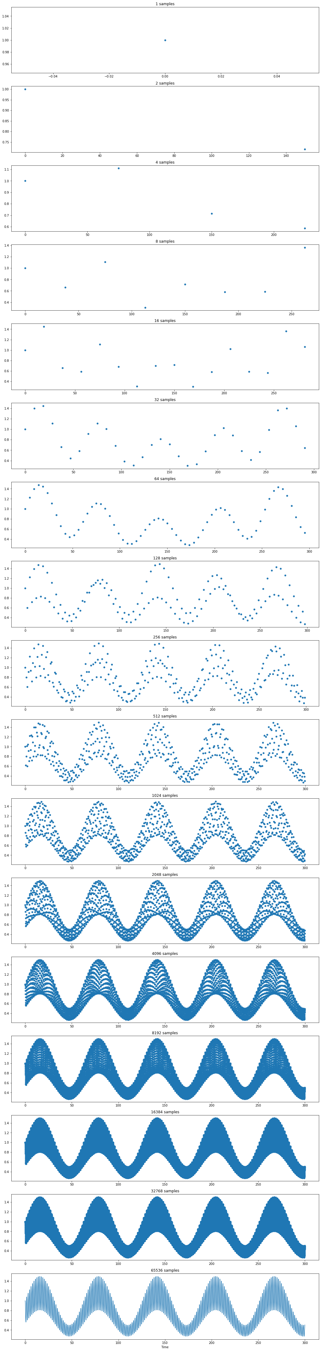
Carefully look over the different ways that sampling can go wrong …
Aliasing .. different signals are indistinguishable when sampled. (Look at the N = 128 chart above … can you see a signal that is not evident at the highest resolution?)
Other examples:
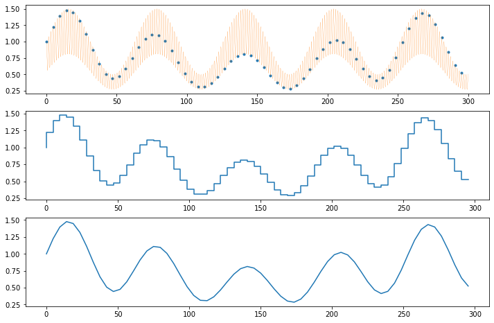
Reconstruction#
Given a series of N samples \(y[n] = y(n\delta)\), \(n = 0, 1, \ldots N-1\), reconstruct a continuous function.
T = 300
N = 64

# sampling
t = np.linspace(0, T, N, endpoint=False)
x = myfun(t)

# create plots
fig, ax = plt.subplots(3, 1, figsize=(12, 8))

# original signal
ax[0].plot(t, x, '.')
t2 = np.linspace(0, T, 10000)
ax[0].plot(t2, myfun(t2), lw=.2)

# step interpolation
ax[1].step(t, x, where="pre")

# linear interpolation
ax[2].plot(t, x)
[<matplotlib.lines.Line2D at 0x7fb5361c7700>]
Anti-aliasing#
What we have to do is eliminate that part of the signal that gets aliased before the sampling. Because if don’t, the aliasing corrupts the signal in ways that can’t be fixed afterwards.
Fourier Analysis#
Complex sinusoids as an Orthonormal Basis#
Fourier analysis begins with specification of a set of countably infinite set of complex valued basis functions for the interval \([0, T]\)
for integer \(k \in (-\infty, \infty)\). Letting \(\bar{phi}_k\) denote the complex conjugate of \(\phi_k\), note that \(\bar{\phi}_k = \phi_{-k}\)
For functions \(f\) and \(g\) defined on the same interval, define the inner product
where \(\bar{f}(t)\) denotes the complex conjugate of \(f(t)\). It’s easy to show the set \(\phi_k(t)\) forms an orthonormal basis under this inner product. First
\begin{align*} \langle \phi_k, \phi_k\rangle & = \frac{1}{T} \int_0^T \bar{\phi}_k(t) \phi_k(t)\ dt \ & = \frac{1}{T} \int_0^T e^{-2\pi i k t/T} e^{2\pi i k t/T}\ dt \ & = \frac{1}{T} \int_0^T dt = 1\ \end{align*}
Then second, for \(k \ne l\),
\begin{align*} \langle \phi_k, \phi_l\rangle & = \frac{1}{T} \int_0^T \bar{\phi}_k(t) \phi_l(t)\ dt \ & = \frac{1}{T} \int_0^T e^{-2\pi i k t/T} e^{2\pi i l t/T}\ dt \ & = \frac{1}{T} \int_0^T e^{2\pi i (l-k)t/T}\ dt \ & = \frac{e^{2\pi i (l-k)t/T}}{2\pi i(l-k)}\bigg|_0^T = \frac{e^{2\pi i (l-k)} - 1}{2\pi i(l-k)} = 0 \qquad \text{for } k\ne l \end{align*}
Next we consider projecting a function \(y\) of \(t\) on the interval \([0, T]\) onto this orthonormal basis.
where \(Y_k\) are the coefficients of expansion. The coeffients are determined
\begin{align*} \langle \phi_k, y\rangle & = \langle \phi_k, \sum_{k’} Y_{k’}\phi_{k’} \rangle = \sum_{k’} Y_{k’}\langle \phi_k, \phi_{k’} \rangle = Y_k \end{align*}
or in closed form as
which computes the Fourier Transform of \(y(t)\) at a countably infinite set of values \(Y_k\).
Application to Real functions#
For real functions \(\bar{y}(t) = y(t)\). As a consequence
\begin{align*} \sum_k \overline{Y_k \phi_k} & = \sum_{k’} Y_{k’} \phi_{k’} \ \sum_k \bar{Y}k \bar{\phi}k & = \sum{k’} Y{k’} \phi_{k’} \ \sum_k \bar{Y}k \phi{-k} & = \sum_{k’} Y_{k’} \phi_{k’} \ \end{align*}
Projecting the left and right hand sides of this equation on the orthonomal basis shows \(\bar{Y}_k = Y_{-k}\) for real functions.
The practical consequence of this is that is not necessary to compute the Fourier coefficients for negative values of \(k\).
Frequency domain interpretation#
The indices \(k\) can be associated with a frequency \(f_k\) where
has units of cycles per unit time. The Fourier coefficients can then be associated with a frequency
where \(f_k = \frac{k}{T}\) for \(k = 0, \pm 1, \pm 2, \ldots\)
Application to Sampled data#
In most applications the function \(f(t)\) is evaluated at regular intervals of time \(t_n = n\delta\). For \(k = 0, \pm 1, \pm 2, \ldots\)
\begin{align*} Y_k & = \frac{1}{T} \int_0^T e^{-2\pi i k t/ T}y(t)\ dt \ & \approx \frac{1}{N\delta} \sum_{n=0}^{N-1} e^{-2\pi i k n \delta / (N\delta)} y_n\delta \ & \approx \frac{1}{N} \sum_{n=0}^{N-1} e^{-2\pi i k n / N} y_n \end{align*}
numpy.fft#
The Numpy library provides a collection of functions to enable use of the Fourier tranform.
%matplotlib inline
import numpy as np
import matplotlib.pyplot as plt
from scipy.fft import fft, ifft, fftfreq
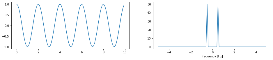
# create time interval and grid
T = 10
N = 100
t = np.linspace(0, T, N, endpoint=False)
# create a function of time
f = lambda t: np.cos(2*np.pi*t*5/T)
def fftplot(ax, t, y):
F = fft(y)
w = fftfreq(len(t), np.mean(np.diff(t)))
s = np.argsort(w)
ax.plot(w[s], np.abs(F[s]))
ax.set_xlabel("frequency [Hz]")
fig, ax = plt.subplots(1, 2, figsize=(16, 3))
ax[0].plot(t, f(t))
fftplot(ax[1], t, f(t))
Examples of Fourier Transforms#
%matplotlib inline
import numpy as np
import matplotlib.pyplot as plt
def fftplot(ax, w, F):
s = np.argsort(w)
ax.plot(w[s], np.abs(F[s]))
from scipy.fft import fft, ifft, fftfreq
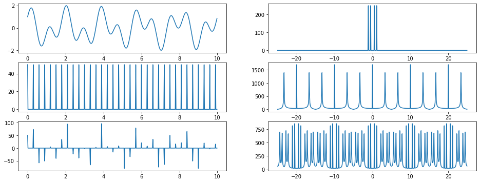
def showfft(t_sample):
# time horizon and sample period
T = 10
dt = 0.02
t = np.linspace(0, T, int(T/dt), endpoint=False)
# function
k = 5
f = lambda t: np.cos(2*np.pi*t*k/T) + np.sin(2*np.pi*t*(k+6)/T)
def delta(t, t_sample):
k = int(t_sample/dt)
return [1/dt if 0 == n % k else 0 for n in range(len(t))]
# compute FFT
F = fft(f(t))
w = fftfreq(len(F), dt)
fig, ax = plt.subplots(3, 2, figsize=(16, 6))
ax[0, 0].plot(t, f(t))
fftplot(ax[0, 1], w, F)
g = delta(t, t_sample)
G = fft(g)
ax[1, 0].plot(t, g)
fftplot(ax[1, 1], w, G)
h = f(t)*delta(t, t_sample)
H = fft(h)
ax[2, 0].plot(t, h)
fftplot(ax[2, 1], w, H)
showfft(0.3)
x = np.zeros(N)
n = np.array(range(0, N))
x[8] = 1

y = fft(x)
k = n

fix, ax = plt.subplots(3, 1, figsize=(8, 12))
ax[0].plot(n, x, '.', ms=10)
ax[1].plot(k, np.abs(y), ms=10)
ax[1].set_title('Fourier Transform')

ax[2].plot(y.real, y.imag, '.')
ax[2].axis("equal")
ax[2].axis("square")

fig.tight_layout()
Euler’s Formula#
Sinusoidal signals#
The complex function
$$
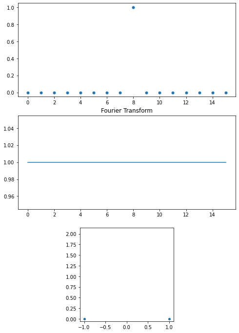
Discrete Fourier Transform#
The Fourier transform is a linear operation \(y = \cal{F}(x)\) where
\begin{align*} y[k] & = \sum_{n=0}^{N-1}e^{-\frac{2\pi}{N} i k n} x[n] \ \text{or} \ y[k] & = \sum_{n=0}^{N-1}\left[\cos\left(\frac{2\pi}{N}kn\right) - i \sin\left(\frac{2\pi}{N}kn\right)\right]x[n] \end{align*}
Each term corresponds to a frequency \(f_{k} = \frac{k}{N}\)
from scipy.fft import fft, ifft

N = 16
x = np.zeros(N)
n = np.array(range(0, N))
x[8] = 1

y = fft(x)
k = n

fix, ax = plt.subplots(3, 1, figsize=(8, 12))
ax[0].plot(n, x, '.', ms=10)
ax[1].plot(k, np.abs(y), ms=10)
ax[1].set_title('Fourier Transform')

ax[2].plot(y.real, y.imag, '.')
ax[2].axis("equal")
ax[2].axis("square")

fig.tight_layout()
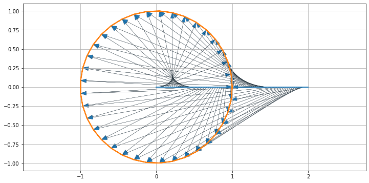
Inverse Discrete Fourier Transform#
The inverse transform is given by
%matplotlib inline

import numpy as np
import matplotlib.pyplot as plt

# create points on the postive x axis
x = np.linspace(0, 2, 75) + 0j
y = np.exp(1j * x * 2 * np.pi)

fig, ax = plt.subplots(1, 1, figsize=(12, 6))
ax.plot(x.real, x.imag, lw=2)
ax.plot(y.real, y.imag, lw=2)

for k in range(len(x)):
    plt.arrow(x[k].real, x[k].imag, y[k].real-x[k].real, y[k].imag-x[k].imag,
             head_width=0.05,length_includes_head=True, lw=.2)

ax.axis('equal')
ax.grid(True)
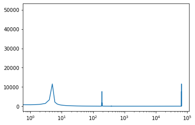
from scipy.fft import fft, ifft

t = np.linspace(0, T, 2**J)
y = fft(x(t))
plt.semilogx(abs(y))
[<matplotlib.lines.Line2D at 0x7fb52d2ff0d0>]