Computer Vision Workflow
Contents
Computer Vision Workflow#
Developing a Process#
Our approach …
Read image
Crop
Separate into channels
Creat a composite
Equalize histogram
Blur/Low Pass Filter
Segment/Threshold
Use Morphology Transforms to isolate objects
Locate Objects - Blobs vs Hough Transforms
Prepare a Report
Python Imports#
We track overall code dependencies by consolidating imports into this cell. Note that we’ll be using elements from multiple packages by relying on the underlying NumPy representation of images to hold the current state of the process.
!pip install opencv-python --upgrade
Requirement already satisfied: opencv-python in /Users/jeff/opt/anaconda3/lib/python3.9/site-packages (4.6.0.66)
Requirement already satisfied: numpy>=1.17.3 in /Users/jeff/opt/anaconda3/lib/python3.9/site-packages (from opencv-python) (1.21.5)
# standard Python libraries
import numpy as np
import matplotlib.pyplot as plt
from PIL import Image
from scipy import ndimage

# computer vision libraries
import cv2 as cv2
Reading images#
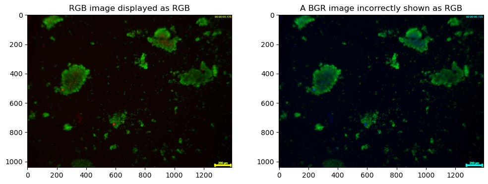
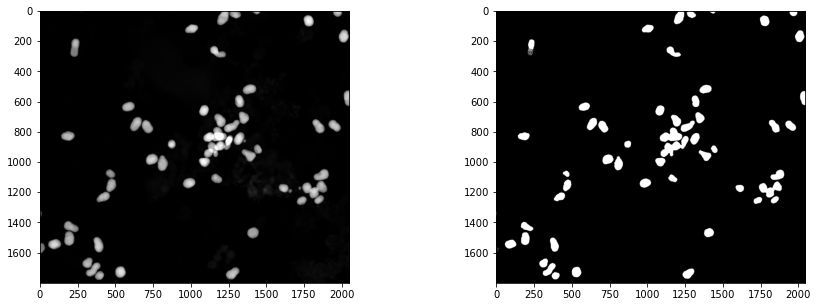
As a first step, read the image, convert to rgb scale, and display. All of these packages have a means of reading raster file images in common formats. There are small (and sometimes frustrating) differences among them. Here we use the Matplotlib imread() method which reads and returns a numpy array.
The array will typical have 2 or 3 dimensions \((h, w, d)\) where \(h\) and \(w\) are image height and width, and \(d\) is pixel depth.
If \(d\) is one or not present, it is a gray scale image
If \(d\) is 3, then typically it is an RGB image with the channels repesenting R, G, and B colors. Note that OpenCV orders the channels as BGR.
If \(d\) is 4, the image could be RGBA where A refers to an alpha transparency channel, or a CYMK encoded color image.
path = "image_data/Burchett Photos/"
file = "Gold STEM HAADF 59000 x 20220318 1542.tif"

path = "image_data/Burchett Photos/"
file = "lowadhesionF_5x_adjustedbrightness-sb.jpg"

# read color image with OpenCV
img_bgr = cv2.imread(path + file)
print(img_bgr.shape)
(1040, 1392, 3)
%matplotlib inline

# convert to RGB
img_rgb = cv2.cvtColor(img_bgr, cv2.COLOR_BGR2RGB)

# display images with Matploblib
fig, ax = plt.subplots(1, 2, figsize=(12, 4))

ax[0].imshow(img_rgb)
ax[0].set_title("RGB image displayed as RGB")

ax[1].imshow(img_bgr)
ax[1].set_title("A BGR image incorrectly shown as RGB")
Text(0.5, 1.0, 'A BGR image incorrectly shown as RGB')
img = img_rgb[20:1000, :, :]
plt.imshow(img)
<matplotlib.image.AxesImage at 0x7fc0d6f6fd90>

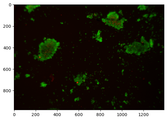
Observations:
There are extraneous elements at the edges of the image
Cropping#
img = img_rgb[0:1800, :, :].copy()
plt.imshow(img)

img = img_rgb[20:1000, :, :]
plt.imshow(img)
<matplotlib.image.AxesImage at 0x7fc0d4bbc040>
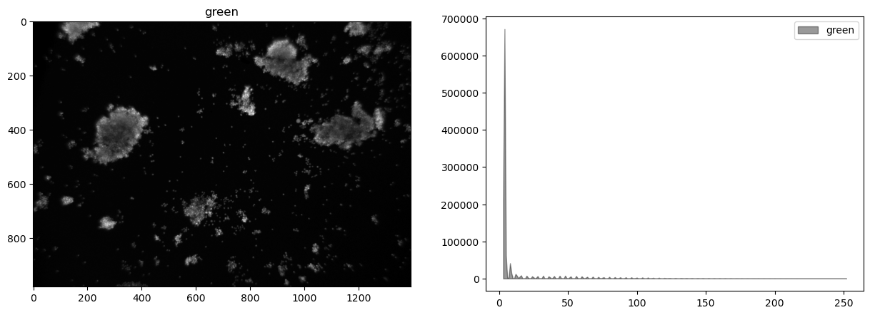
Channels and Histograms#
An image is comprised of one or more channels
Each channel can be treated as a gray scale image
The values at each pixel may be
An 8-bit unsigned integer in the range 0 to 255 (most common)
A 12, 14, or 16 bit unsigned integer
A real number between 0 and 1
Color must always be interpreted with respect to color space.
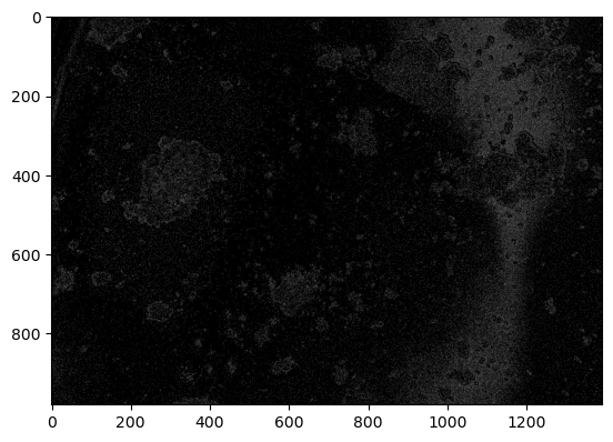
r, g, b = cv2.split(img)
r[r <= 50] = 0
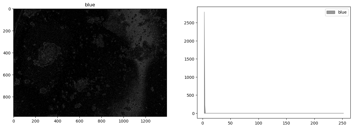
plt.imshow(b, cmap="gray")
<matplotlib.image.AxesImage at 0x7fc0d5340e20>
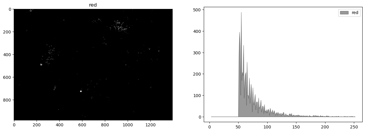
Histograms are a tool for analyzing the distribution of gray levels in a channel. It’s a powerful tool for controlling exposure and processing images for presentation.
def histogram(channel, bp=3, wp=252):
"""Return histogram and bins for a single channel."""
hist = cv2.calcHist([channel], [0], None, [wp-bp+1], [bp, wp])
bins = np.array([b for b in range(bp, wp+1)])
return hist.flatten(), bins
def display_channel(channel, label=""):
fig, ax = plt.subplots(1, 2, figsize=(15, 5))
ax[0].imshow(channel.astype(np.uint8), cmap="gray")
ax[0].set_title(label)
hist, bins = histogram(channel.astype(np.uint8))
ax[1].fill_between(bins, hist, alpha=0.4, color="k", label=label)
ax[1].legend()
display_channel(r, "red")
display_channel(g, "green")
display_channel(b, "blue")
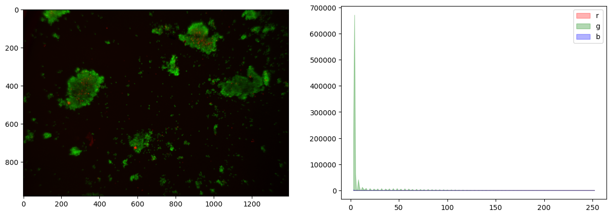
fig, ax = plt.subplots(1, 2, figsize=(15, 5))
ax[0].imshow(img)
for color, channel in zip(['r', 'g', 'b'], [r, g, b]):
hist, bins = histogram(channel)
ax[1].fill_between(bins, hist, color=color, label=color, alpha=0.3)
ax[1].legend()
<matplotlib.legend.Legend at 0x7fc0d7dde730>
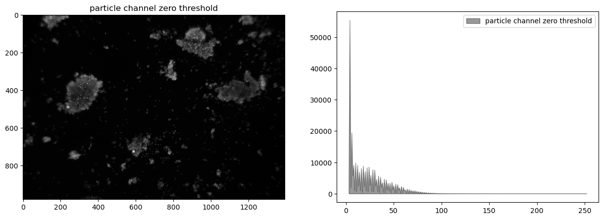
Creating a composite channel#
This image shows very little difference among the color channels.
# subtract blue channel from green channel
cimg = (0.5*r + 0.5*g)

# convert to integer
cimg = cimg.astype(np.uint8)
display_channel(cimg, "particle channel zero threshold")
Histogram equalization#
At this stage our composite image appears significantly underexposed. Looking at just the green channel, increasing the exposure 4x, or even 6x, would significantly brighten the particles that we’re seeking to detect. In future versions of the experiment it may be useful to experiment with signficantly brighter lenses, light sources, or longer exposures.
In the meanwhile, the step in image processing is to equalize the histogram to improve opportunities for effective particle detection.
himg = cv2.equalizeHist(cimg)
display_channel(himg, 'equalized')
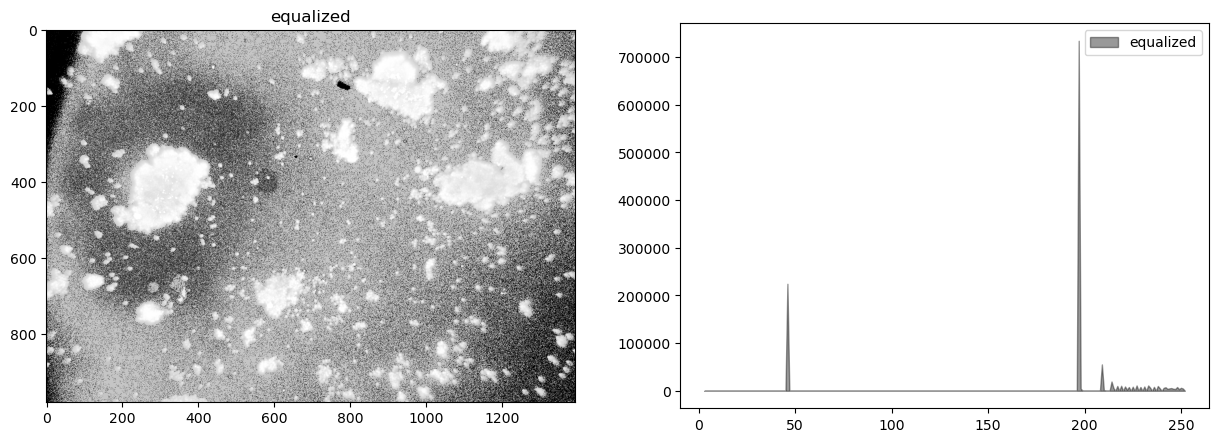
Observations
Quantization (sometimes seen as banding) caused by limited number of levels in the channel.
The image was underexposed at the time of capture.
There is significant and probably irrelevant information buried in the dark tones.
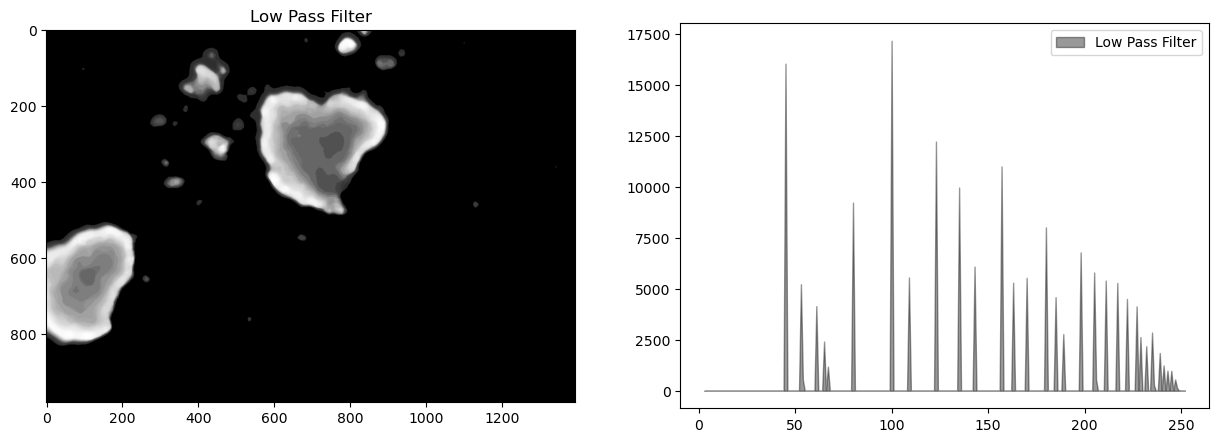
Blur filter#
# kernel size (odd number)
ksize = 21

# median filter
bimg = cv2.medianBlur(himg, ksize)
display_channel(bimg, "Low Pass Filter")
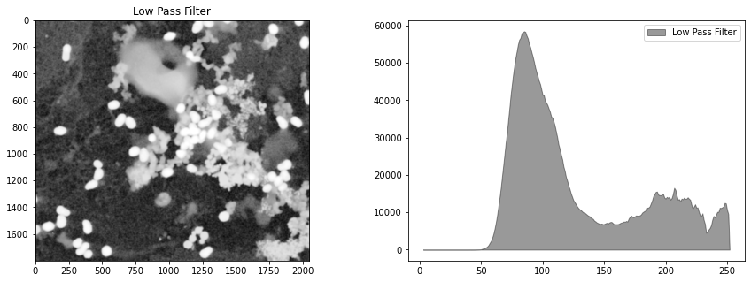
# Gaussian filter
bimg = cv2.GaussianBlur(himg, (ksize, ksize), 0)
display_channel(bimg, "Low Pass Filter")
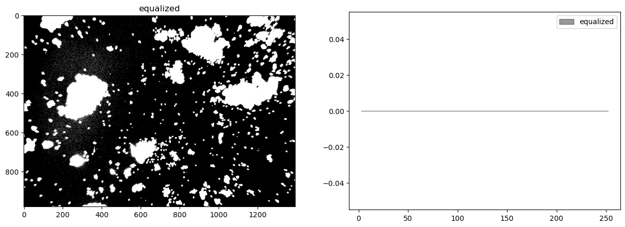
Thresholding/Segmentation#
The purpose of threshold is to isolate the features of interest from background noise.
https://docs.opencv.org/3.4/d7/d4d/tutorial_py_thresholding.html
ret, timg = cv2.threshold(himg, 200, 255, cv2.THRESH_BINARY)
display_channel(timg, 'equalized')
threshold = 130

T, simg = cv2.threshold(timg, 0, 255, cv2.THRESH_OTSU + cv2.THRESH_BINARY)

fig, ax = plt.subplots(1, 2, figsize=(15, 5))
ax[0].imshow(img)
ax[1].imshow(simg, cmap="gray")
print(f"Threshold = {T}")
Threshold = 0.0
Morphological Transformation#
The next goal is to remove noise and to separate particles.
kernel = np.ones((3, 3))
iterations = 8

def morph_close (img, kernel, iterations=1):
    ret = cv2.dilate(img, kernel=kernel, iterations=iterations)
    ret = cv2.erode(ret, kernel=kernel, iterations=iterations)
    return ret

close_img = morph_close(simg, kernel, iterations)
plt.imshow(close_img, cmap="gray")
<matplotlib.image.AxesImage at 0x7fbd7290dc70>
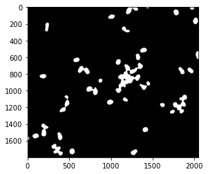
kernel = np.ones((3, 3))
iterations = 8

def morph_open(img, kernel, iterations):
    ret = cv2.erode(img, kernel=kernel, iterations=iterations)
    ret = cv2.dilate(ret, kernel=kernel, iterations=iterations)
    return ret

open_img = morph_open(close_img, kernel, iterations)

plt.imshow(open_img, cmap="gray")
<matplotlib.image.AxesImage at 0x7fbd728ebac0>

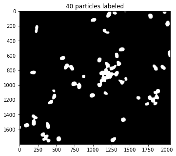
Finding Objects#
http://pageperso.lif.univ-mrs.fr/~francois.denis/IAAM1/scipy-html-1.0.0/tutorial/ndimage.html
# find particles and plot objects
structure = np.ones((3, 3))
label_img, particle_count = ndimage.measurements.label(open_img, structure=structure)

# pixels are labeled with numbers corresponding to objects
fig, ax = plt.subplots(1, 1, figsize=(8, 5))
ax.imshow(np.where(label_img > 0, 1, np.zeros(label_img.shape)), cmap="gray")
ax.set_title(f"{particle_count} particles labeled")
/var/folders/cm/z3t28j296f98jdp1vqyplkz00000gn/T/ipykernel_11775/3620703114.py:3: DeprecationWarning: Please use `label` from the `scipy.ndimage` namespace, the `scipy.ndimage.measurements` namespace is deprecated.
  label_img, particle_count = ndimage.measurements.label(open_img, structure=structure)
Text(0.5, 1.0, '40 particles labeled')
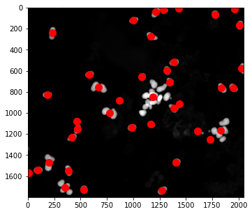
# centers of mass
pts = ndimage.center_of_mass(open_img, label_img, np.arange(1, particle_count + 1))

x = [x for (y,x) in pts]
y = [y for (y,x) in pts]

fig, ax = plt.subplots(1, 1, figsize=(8, 5))
ax.imshow(img)
ax.plot(x, y, '.', ms=20, color='r')
[<matplotlib.lines.Line2D at 0x7fbd81a7d8e0>]
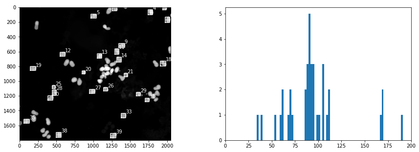
Finding and Displaying Particles#
# find the objects and place bounding boxes
slices = ndimage.find_objects(label_img)
sizes = [np.sqrt((b.stop-b.start)**2 + (a.stop-a.start)**2) for a,b in slices]


fig, ax = plt.subplots(1, 2, figsize=(15, 5))
ax[1].hist(sizes, bins=200)
ax[1].set_xlim(0, 200)
ax[0].imshow(img)
for k,size in enumerate(sizes):
    if size > 50 and size < 100:
        a,b = slices[k]
        ya = a.start
        yb = a.stop
        xa = b.start
        xb = b.stop
        ax[0].plot([xa, xb, xb, xa, xa], [yb, yb, ya, ya, yb], 'w')
        ax[0].text(xb, ya, f"{k}", color="w")
Creating a Training Set#
kdx = [k for k, size in enumerate(sizes) if size > 50 and size < 100]

dx = 100
dy = 100

def round_slice(s, n):
    """Round up slice to be width n"""
    m = s.stop - s.start
    start = s.start - int((n - m)/2)
    stop = start + n
    return slice(start, stop, 1)

fig, ax = plt.subplots(len(kdx), 1, figsize=(5, 5*len(kdx)))
for i, k in enumerate(kdx):
    a, b = slices[k]
    ax[i].imshow(open_img[round_slice(a, 100), round_slice(b, 100)])
/var/folders/cm/z3t28j296f98jdp1vqyplkz00000gn/T/ipykernel_11775/1243267172.py:16: UserWarning: Attempting to set identical bottom == top == -0.5 results in singular transformations; automatically expanding.
  ax[i].imshow(open_img[round_slice(a, 100), round_slice(b, 100)])

What did we learn about our application?#
Improved Image Capture
Reduce glare from the blue leds
Increase exposure
Image Processing Steps
read image
separate channels
combine channels to isolate green flourescent particles (weights?)
median filtering (size?)
histogram equalization
threshold (threshold value?)
morphological opening (kernal?, iterations?)
labeling (size?)