Basics of Linear DC Circuits
Contents
Basics of Linear DC Circuits#
Dimensions and Units#
Ampere (A) In November 2018, several of the SI base units were redefined in terms that finally eliminated the use of artifacts. In the new system, the Ampere is the flow of one Coulomb \(C\) per second, where the numerical value of elementary charge \(e\) of an electron is fixed as \(1.602176634 \times 10 ^{-19}\)C
Volt (V) An electric field exerts force on an electric charge, therefore work is being done when a current passes through an electric field. Volts measure the magnitude of an electric field such that one volt is the potential field that produces 1 Watt of power for an electric current of 1 Ampere.
Power (P) Power, measued in units of Watts, is the amount of work done per unit time. By definition of Volt,
Kirchhoff’s rules#
The circuits used in laboratory instrumentation are comprised of lumped elements such as conductors, resistors, capacitors, inductors, and various semiconductor components. Kirchhoff’s rules are the foundation of circuit analysis for lumped elements. There are two basic rules:
Kirchhoff’s current rule. Given a node in a circuit, the algebraic sum of currents is zero. That is, $\(\sum_{n=1}^N I_n = 0\)\( where \)I_n\( is the signed (i.e., positive or negative) current in the \)n^{th}$ branch of the node.
Kirchoff’s voltage rule. The sum of potential differences is zero around any closed loop. That is $\(\sum_{n=1}^NV_n = 0\)\( where \)V_n$ is the signed (i.e, positive or negative) potential difference across each device in the closed loop.
These rules are the foundation for circuit analysis, but do depend on several key assumptions that do not hold in for all laboratory situations. In particular, these rules assume a circuit can be modeled as lumped elements that do not interact through electric or magnetic fields. These assumptions may be violated, for example, in high frequency transmission lines where charge density may be oscillating, or where there is significant interaction of electrical or magnetic fields with the surrounding environment. Since these types of interactions can occur in a laboratory setting, one needs to be aware of the limits of basic circuit analysis.
Ohm’s law#
Ohm’s law is a linear consituitive equation describing the relationship between current density \(\bf j\), electric field \(\bf e\), and magnetic flux density \(\bf b\) for a bulk conductors. In vector notation
where \(\bf v\) is velocity and \({\bf j}_s\) is any current source imposed independently of an electromagnetic field. In this case \(\sigma\) is a conductivity tensor for anisotropic materials.
For isotopic conductors where there is no motion relative to a magnetic field, and no other current flux imposed independently of an electric field, Ohm’s law simplifies to the scalar equation
where the parameter \(\sigma\) is a scalar conductivity measured in units of Siemens/meter (S/m), \(e\) is electric field measured in volts/meter, and \(j\) is current density measured in Amperes per square meter. The resistivity \(\rho\) of the material is
which has units of ohms per meters.
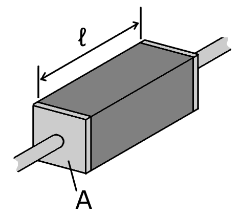
When working with electronic components we are working with specimens of a particular material. For a device with cross-sectional area \(A\) and length \(l\), the resistance of the specimen is given by Pouillet’s law
which has units of \(ohms\). Defining current as \(I = j A\) and electric field as \(e = V/l\) results in Ohm’s law as it is commonly encountered in electronic circuit analysis.
Ideal Voltage and Current Sources#
An ideal voltage source is a device that maintains a fixed voltage regardless of the current required by the load.

Given \(V\) and \(R\), the current flow \(I = V/R\), and power is \(P = V I = V^2/R\). Obviously this idealization breaks down in the limit \(R = 0\) which would require an infinite and therefore infeasible amount of current.
An ideal current source is a device providing a fixed current regardless of the load or resistance imposed on the source.

Given \(I\) and \(R\), the voltage is \(V = I R\) and power is \(P = V I = I^2 R\). This idealization breaks down in the limit \(R = \infty\) which would require infinite voltage to impose a finite current.
Most common power supplies are set up as voltage sources with some sort of current limit.
Resistor Networks#
Systems comprised of interconnected resistors can be analyzed using the Kirchhoff circuit laws.
Voltage Divider#

\begin{align*} V_{in} & = V_1 + V_2 \ & = I R_1 + I R_2 \ \end{align*}
Capacitors#
An ideal capacitor
where \(C\) is capacitance measured in Farads. A current of 1 ampere would produce a 1 volt/sec increase in voltage for a 1 Farad capacitor. 1 Farad is a lot of capacitance!
Alternatively,
From this we see that a capacitor stores charge. The voltage increases as more charge is stored. The units of farads are coulombs per volt.
Using Laplace transforms with zero initial conditions,
Drawing a parallel with Ohm’s law, we see that \(\frac{1}{Cs}\) is the complex impedence of a capacitor.
Inductors#
An ideal inductor creates a counter potential as a result of increasing current.
In a qualititative sense, an inductor resists a change in current. The work being done on the inductor to move current through the device is being stored in the magnetic field. The energy stored in the electric field is returned to the circuit when vol